11. Storm Surge emulator#

inputs required:

Historical DWTs
Historical SLP
Synthetic DWTs

in this notebook:

Obtain historical storm surge as the inverse barometer
Simulation of storm surge for each synthetic DWT (daily resolution)

Workflow:

TITLE

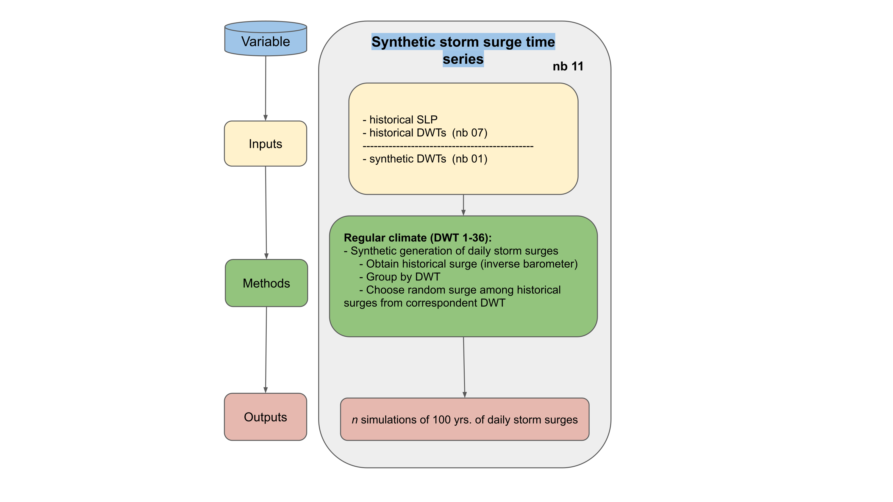
The offshore storm surge can be approximated as the inverse barometer effect: A decrease in atmospheric pressure of 1 mb will produce an increase in sea level of around 1 cm.

The storm surge generated by the wind set-up will only be considered at nearshore locations.

The synthetic generation of surge conditions on a regular climate (DWT1-36) is made by randomly selecting one of the historical surge conditions for each DWT.

#!/usr/bin/env python
# -*- coding: utf-8 -*-

# common
import os
import os.path as op
import glob

# pip
import numpy as np
import xarray as xr
import pandas as pd
from datetime import datetime
import matplotlib.pyplot as plt
from matplotlib import gridspec

# DEV: override installed teslakit
import sys
sys.path.insert(0, op.join(os.path.abspath(''), '..', '..', '..'))

# teslakit
from  bluemath.teslakit.io.aux_nc import StoreBugXdset

11.1. Files and paths#

# project path
p_data = '/Users/albacid/Projects/TeslaKit.2.0_projects/SAMOA'
p_out = op.join(p_data,'TIDE')

# input files
dwt_his_file = op.join(p_data,'ESTELA','pred_slp_grd','kma.nc')  
dwt_sim_file = op.join(p_data,'ESTELA','DWT_sim.nc')  
slp_his_file = op.join(p_data,'resources','SLP_hind_daily_wgrad.nc')

# output files
IB_his_file = op.join(p_out, 'IB_noTCs_daily_his.nc')
IB_sim_file = op.join(p_out, 'IB_noTCs_daily_sim.nc')

11.2. Parameters#

site = 'samoa'
#pnt_lon = -172.07+360  (187.93)
#pnt_lat = -13.76
lonp = 187 # closest coordinates in SLP dataset
latp = -14

SLP_his = xr.open_dataset(slp_his_file)
DWTs_his = xr.open_dataset(dwt_his_file)
DWTs_sim = xr.open_dataset(dwt_sim_file)


DWTs_his = xr.Dataset({'bmus':(('time'), DWTs_his.sorted_bmus_storms.values.astype(int))},
    coords = {'time':(('time'), DWTs_his.time.values)})

n_clusters = 42

11.3. Obtain historical IB#

SLP_his = SLP_his.sel(time=slice(DWTs_his.time.values[0], DWTs_his.time.values[-1]))

# --------------------------------------
# Inverse Barometer (IB)

# select closest grid point to Site
IB_his = SLP_his.sel(longitude = lonp, latitude = latp) 

# Calculate anomalies and change units 
IB_his['slp'] = IB_his.slp*0.01 # (Pa to mb)
IB_his['slp_anomaly'] = IB_his.slp - np.mean(IB_his.slp.values)
IB_his['level_IB'] = -1*IB_his.slp_anomaly # (Inverse Barometer: mb to cm)
IB_his['level_IB'] = IB_his.level_IB/100.0 # (cm to m)


# Add DWT to dataset
IB_his['DWT'] = DWTs_his.bmus

IB_his = IB_his.drop({'slp','slp_gradient','slp_anomaly' })

# save
IB_his.to_netcdf(IB_his_file)

IB_his = xr.open_dataset(IB_his_file)

11.4. IB emulator#

# Define output
IB_sim = DWTs_sim.copy(deep=True)
IB_sim['level_IB']=(('time','n_sim'), np.zeros((len(DWTs_sim.time), len(DWTs_sim.n_sim) ))*np.nan)

# Group historical IB data by DWT
IB_his_dwts = np.zeros((n_clusters,len(IB_his.time)))*np.nan
for dd in range(n_clusters):
    IB_his_dd = IB_his.where(IB_his.DWT==dd, drop=True)    
    IB_his_dwts[dd,:len(IB_his_dd.time)] = IB_his_dd.level_IB.values

# Simulate
for n in DWTs_sim.n_sim:
    print('- Sim: {0} -'.format(int(n)+1))
    
    # Select simulation of DWTs
    DWTs_sim_n = DWTs_sim.isel(n_sim=n)

    for ind_t, dwt in enumerate(DWTs_sim_n.evbmus_sims.values):
            
        # select randomly one historical value for that DWT (including TCs in case it doesn't enter r2)
        IB_his_dwt = IB_his_dwts[int(dwt-1),:]
        IB_his_dwt = IB_his_dwt[~np.isnan(IB_his_dwt)]

        rnd_t = np.random.randint(0, len(IB_his_dwt))

        IB_sim['level_IB'][ind_t,n] = IB_his_dwt[rnd_t]
        
# save    
StoreBugXdset(IB_sim, IB_sim_file)
              

11.5. Validation#

IB_sim = xr.open_dataset(IB_sim_file)

# choose simulation to plot
n = 0
IB_sim_n = IB_sim.isel(n_sim=n)

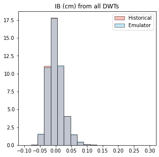
# All DWTs

plt.figure(figsize=(5,5))

n_bins = np.linspace(-0.1,.3,20)
plt.hist(IB_his.level_IB, n_bins,density=True,label='Historical',color='salmon',alpha=0.5,edgecolor='black');
plt.hist(IB_sim_n.level_IB, n_bins,density=True,label='Emulator',color='skyblue',alpha=0.5,edgecolor='black');
plt.legend()
plt.title('IB (cm) from all DWTs');

import warnings
warnings.filterwarnings('ignore')

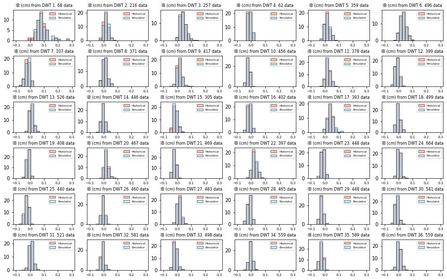
# For each DWT

n_bins = np.linspace(-0.1,.3,20)

fig = plt.figure(figsize=[15.6,11.4])
gs = gridspec.GridSpec(7, 6, hspace=0.5) #, wspace=0.0, hspace=0.0)
gr, gc = 0, 0

for dwt in range(0,36):

    IB_his_dwt = IB_his.level_IB.where(IB_his.DWT==dwt, drop=True)
    IB_sim_n_dwt = IB_sim_n.level_IB.where(IB_sim_n.evbmus_sims==dwt+1, drop=True)
    
    ax = plt.subplot(gs[gr, gc])

    ax.hist(IB_his_dwt, n_bins,density=True,label='Historical',color='salmon',alpha=0.5,edgecolor='black');
    ax.hist(IB_sim_n_dwt, n_bins,density=True,label='Emulator',color='skyblue',alpha=0.5,edgecolor='black');
    ax.legend(prop={'size':6})
    ax.set_title('IB (cm) from DWT ' + str(dwt+1) + '. ' + str(len(IB_his_dwt)) + ' data', fontsize=8)
    ax.set_xticks([-.1,0,.1,.2,.3])
    plt.xticks(fontsize=7)

    # counter
    gc += 1
    if gc >= 6:
        gc = 0
        gr += 1
    
    

Storm Surge emulator

Contents