Anual Weather Types
Contents
1. Anual Weather Types#
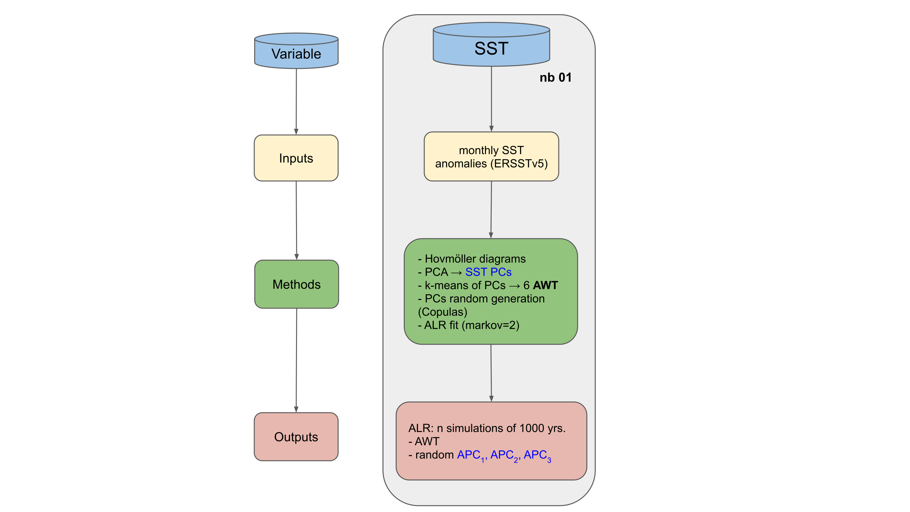
Obtain Anual Weather Types (AWT) following the methodology explained in Anderson et al. (2019)
inputs required:
Sea Surface Temperature Anomalies (SSTA) extracted from the Extended Reconstructed Sea Surface Temperature v5 (ERSSTv5; Huang et al., (2015)). Rectangular region from 120°E to 280°E and 5°N to 5°S
in this notebook:
Construct SSTA Hovmöller diagrams
Perform PCA to the Hovmöller diagrams
K-means to the PCA obtaining 6 AWT
Synthetic generation of tri-variate annual PCs (APC1,APC2, and APC3)
Synthetic generation of AWT based on a second-order markov chain
Workflow:
#!/usr/bin/env python
# -*- coding: utf-8 -*-

# common
import os
import os.path as op
import pickle
from datetime import datetime

# pip
import xarray as xr
import numpy as np

# DEV: override installed teslakit
import sys
sys.path.insert(0, op.join(os.path.abspath(''),  '..','..', '..','..'))

# teslakit
from bluemath.teslakit2.toolkit.pca import PCA_LatitudeAverage
from bluemath.teslakit2.toolkit.kma import kma_simple
from bluemath.teslakit2.toolkit.statistical import copula_simulation

from bluemath.teslakit2.io.aux import save_nc
from bluemath.teslakit2.util.time_operations import xds_reindex_daily, xds_reindex_monthly

from bluemath.teslakit2.toolkit.alr import ALR_WRP

from bluemath.teslakit2.plotting.awt import Plot_AWTs_EOFs, Plot_AWTs, Plot_AWTs_Dates, Plot_AWTs_Validation
from bluemath.teslakit2.plotting.pcs import Plot_PCs_Compare_3D, Plot_PCs_WT
1.1. Files and paths#
# project path
p_data =  r'/media/administrador/HD2/SamoaTonga/data'
site = 'Samoa'
p_site = op.join(p_data, site)

# deliverable folder
p_deliv = op.join(p_site, 'd09_TESLA')

# output path
p_out = op.join(p_deliv,'SST')
if not os.path.isdir(p_out): os.makedirs(p_out)


# input data
sst_file = op.join(p_deliv,'resources','SST_1854_2021_Pacific.nc')

# output data
sst_pca_file = op.join(p_out,'SST_PCA.nc') # PCA results
sst_awt_file = op.join(p_out,'SST_KMA.nc') # KMA results
SST_dPCs_fit_file = op.join(p_out,'SST_dPCs_fit.pickle') # PCs used for fitting the gaussian copulas
SST_dPCs_rnd_file = op.join(p_out,'SST_dPCs_rnd.pickle') # PCs obtained with copula simulation
alr_path = op.join(p_out,'alr_w') # path to store ALR results
sst_awt_sim_file = op.join(p_out,'SST_AWT_sim.nc') # AWTs obtained with ALR
pcs_sim_file = op.join(p_out,'SST_PCs_sim.nc') # Generated PCs for above AWTs
pcs_sim_m_file = op.join(p_out,'SST_PCs_sim_m.nc') # PCs resampled to monthly
pcs_sim_d_file = op.join(p_out,'SST_PCs_sim_d.nc') # PCs resampled to daily
1.2. Parameters#
# --------------------------------------
# load data and set parameters

SST = xr.open_dataset(sst_file)  # SST Predictor
var_name = 'sst'

# SST Predictor PCA parameters
pca_year_ini = 1880
pca_year_end = 2020
pca_month_ini = 6
pca_month_end = 5
num_clusters = 6
repres = 0.95

# ALR parameters
alr_markov_order = 2

# PCs copula generation parameters (PCs 1, 2, 3)
num_PCs_rnd = 1000
kernels = ['KDE', 'KDE', 'KDE']

# Simulation
num_sims = 100
y1_sim = 2020
y2_sim = 2101
1.3. SST - Principal Components Analysis#
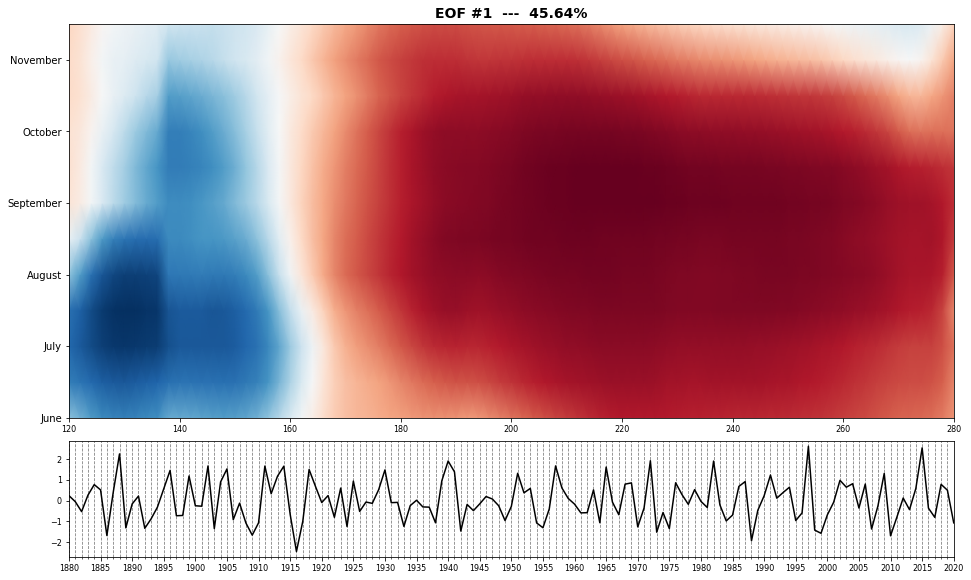
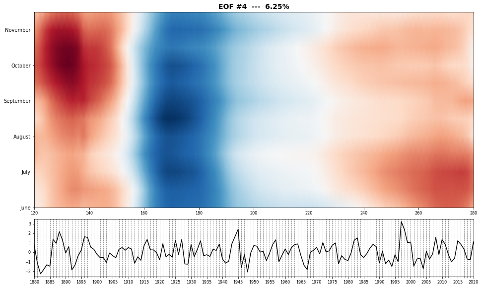
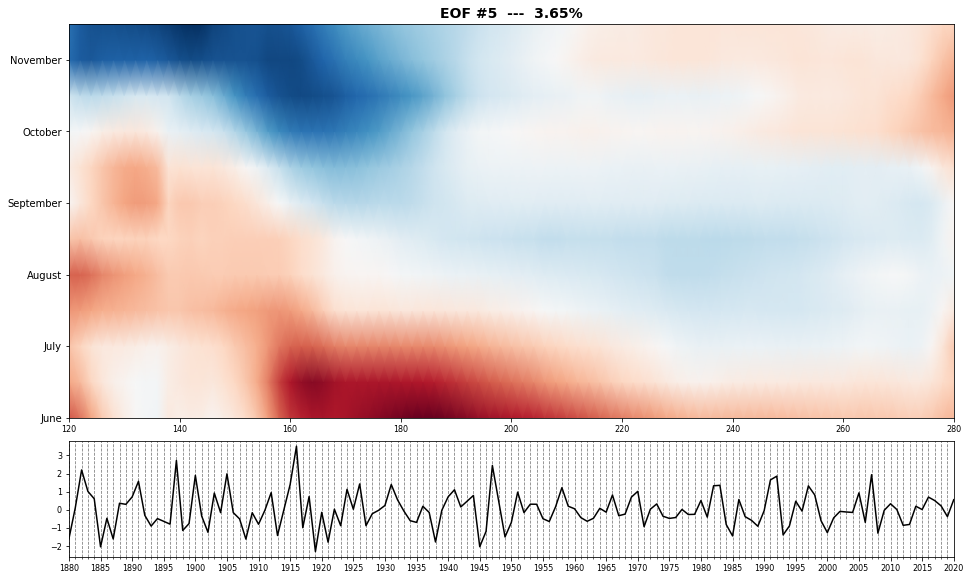
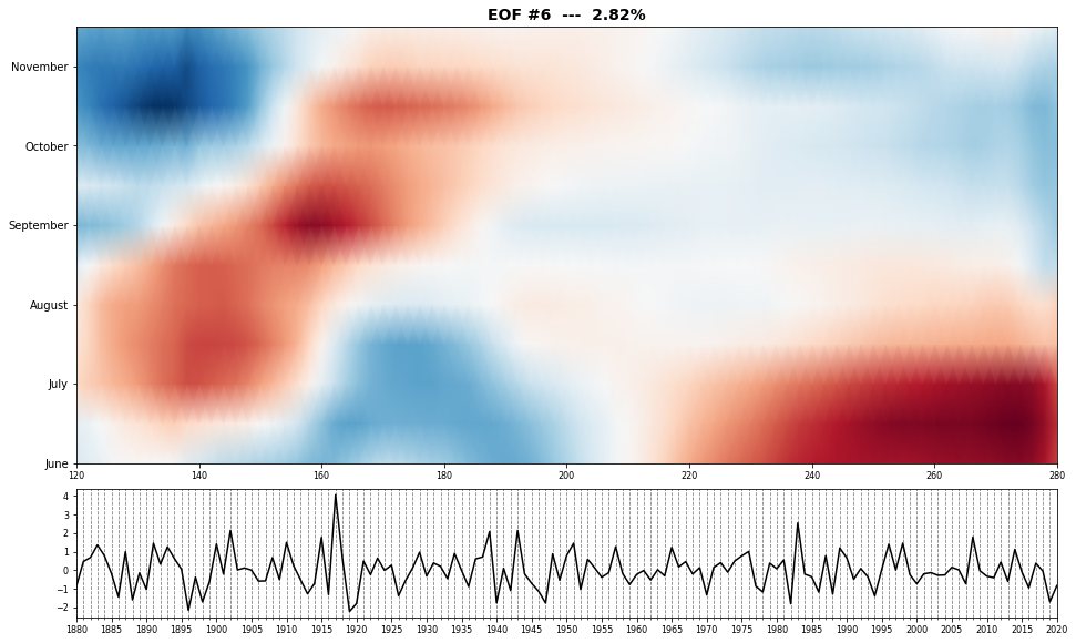
Anomalies are computed by removing 11-year running averages for each month at every node. The monthly longitudinal location of anomalously warm water and its temporal behavior during the year was preserved in the AWT by averaging monthly SSTA values at each longitude to construct Hovmöller diagrams (Hovmöller, 1949). Each diagram begins in June and ends in the following May to capture SSTA variability throughout the boreal winter.
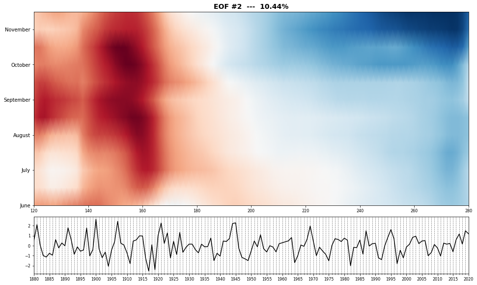
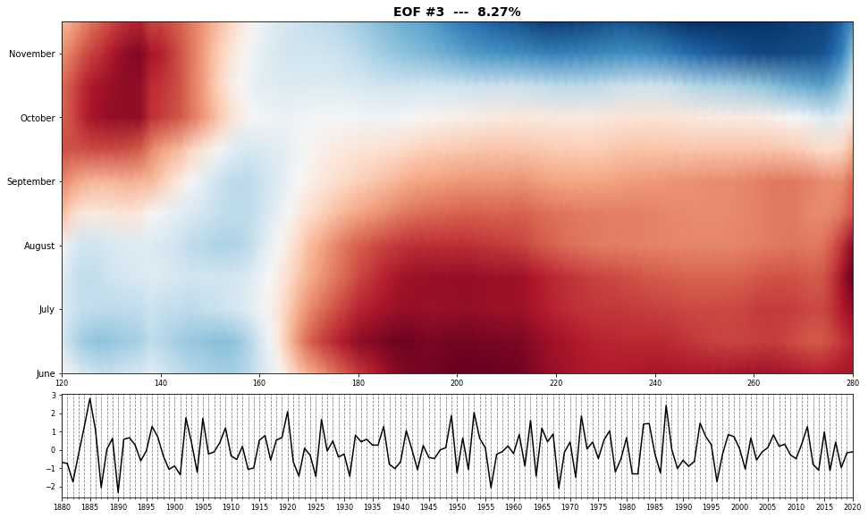
EOF1 explains 48% of the variance, predominantly related to the seesaw effect of warm water anomalies located either east or west of 165°E. The yearly PC values of EOF1 strongly correlate with the average annual ONI (R2=0.94) and average annual NINO3.4 (R2=0.91) indices, indicating that the PCA of Hovmöller space captures the same dominant interannual variability identified by classical ENSO indices. EOF2 (11% of the variance) is predominantly associated with shifting seasonal anomalies in the east Pacific, while EOF3 (8% of the variance) exhibits a temporal and spatial pattern akin to a Kelvin wave of an SSTA propagating west to east during northern hemisphere summer and fall (see figures below).
# --------------------------------------
# Principal Components Analysis SST data

# PCA (anomalies, latitude average)
SST_PCA = PCA_LatitudeAverage(SST, var_name, pca_year_ini, pca_year_end, pca_month_ini, pca_month_end);

# store SST PCs
save_nc(SST_PCA, sst_pca_file)
# PCA data for plots

lon  = SST_PCA.pred_lon.values[:]
PCs  = SST_PCA.PCs.values[:]
EOFs = SST_PCA.EOFs.values[:]
vari = SST_PCA.variance.values[:]
time = SST_PCA.time.values[:]
# Plot first 6 EOFs

Plot_AWTs_EOFs(PCs, EOFs, vari, time, lon, 6);
1.4. SST - KMeans Classification –> Annual Weather Types#
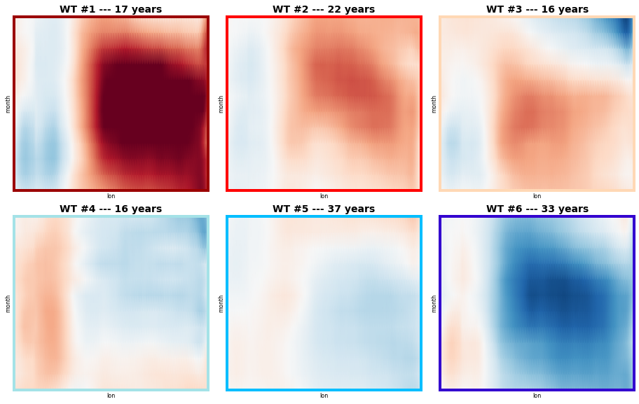
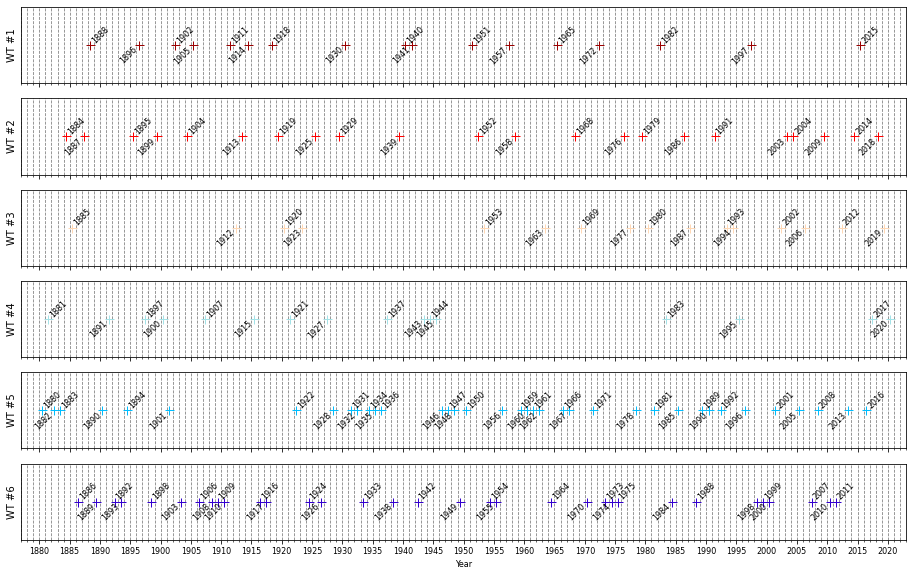
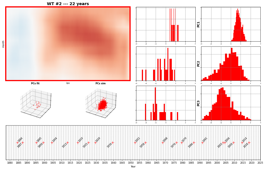
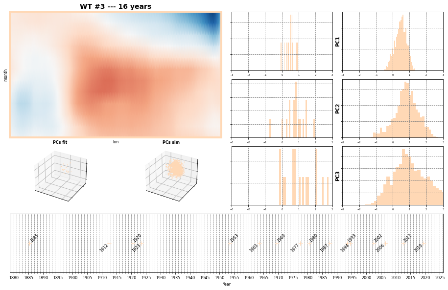
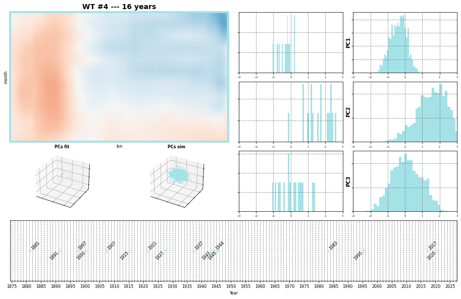
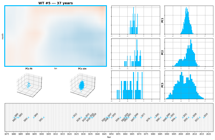
The Annual PCs are classified into 6 representative clusters based on k-means algorithm, defined as Annual Weather Types (AWTs)
Annual weather type #1 (AWT#1) clusters years of positive SSTA in the east Pacific, which are representative of canonical El Niño years and includes the classic examples of 1982-83, 1997-98, and 2015-16. AWT#2 clusters Modoki El Niño years, with the largest anomalies slightly further west along the equator than AWT#1, and identifies such Modoki years as 1994-95, 2002-03, and 2009-10 (Ashok et al., 2007). The opposite end of the spectrum is AWT#6, which exhibits negative SSTA in the east Pacific representative of La Niña years. Other ENSO states identified by the clustering method are interpreted as transition years between the El Niño/La Niña extremes. AWT#3 identifies increasing positive SSTA throughout the year and often occurred prior to El Niño, while AWT#4 exhibits the opposite SSTA behavior and is a precursor to La Niña.
# --------------------------------------
# KMA Classification

SST_AWTs = kma_simple(SST_PCA, num_clusters, repres)
print(SST_AWTs)

# store SST AWTs
save_nc(SST_AWTs, sst_awt_file)
Number of PCs: 141
Number of PCs explaining 95.0% of the EV is: 27
<xarray.Dataset>
Dimensions:     (n_clusters: 6, n_features: 28, n_pcacomp: 141, n_pcafeat: 972)
Dimensions without coordinates: n_clusters, n_features, n_pcacomp, n_pcafeat
Data variables:
    bmus        (n_pcacomp) int64 4 3 4 4 1 2 5 1 0 5 4 ... 5 2 4 1 0 4 3 1 2 3
    cenEOFs     (n_clusters, n_features) float64 37.3 -5.132 ... -0.03938
    centroids   (n_clusters, n_pcafeat) float64 -0.4457 -0.5859 ... -0.2807
    Km          (n_clusters, n_pcafeat) float64 -0.1204 -0.1614 ... -0.2422
    group_size  (n_clusters) int64 17 22 16 16 37 33
    PCs         (n_pcacomp, n_features) float64 4.998 4.939 ... -2.453 0.08764
    variance    (n_pcacomp) float64 446.7 102.2 81.0 ... 2.123e-05 2.06e-30
    time        (n_pcacomp) datetime64[ns] 1880-06-01 1881-06-01 ... 2020-06-01
# KMA data for plots
bmus = SST_AWTs.bmus.values[:]
time = SST_AWTs.time.values[:]
Km   = SST_AWTs.Km.values[:]
# Plot Annual Weather Types
Plot_AWTs(bmus, Km, num_clusters, lon);
# Plot year/label AWTs
Plot_AWTs_Dates(bmus, time, num_clusters);
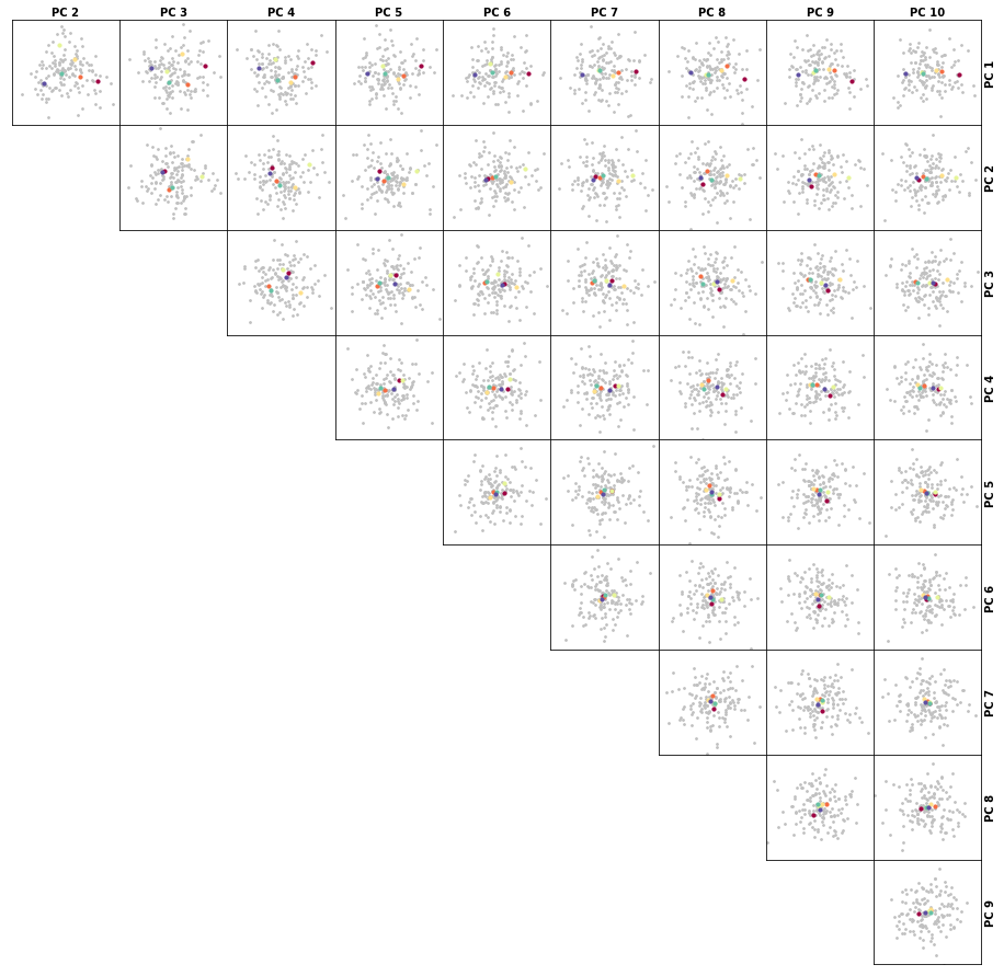
# Plot PCs with AWTs centroids
Plot_PCs_WT(PCs, vari, bmus, num_clusters, n=10);
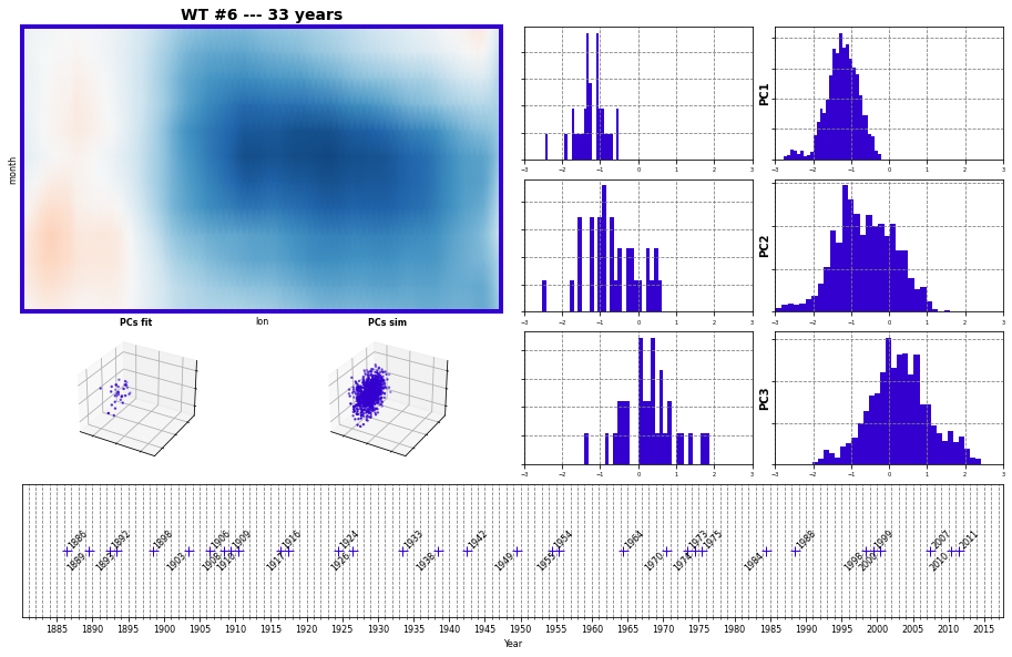
1.5. Synthetic AWT#
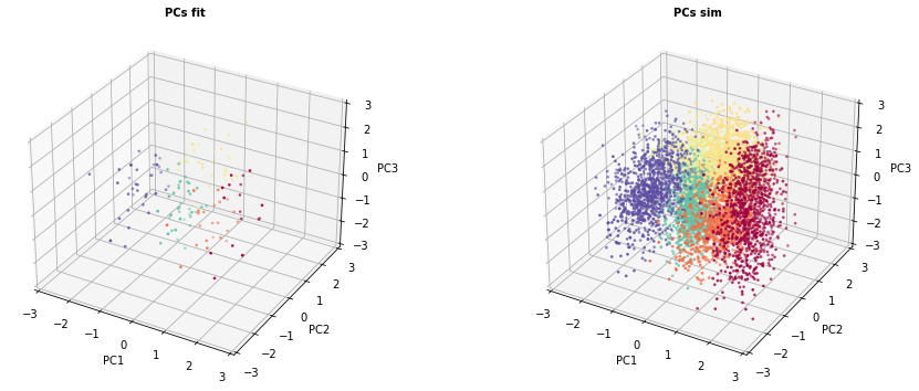
Categorical AWTs were converted to principal component space by defining tri-variate gaussian copulas (e.g. Wahl et al., 2012; Masina et al., 2015) for each AWT using the marginal distributions of its respective three PC components APC1, APC2, and APC3. Each simulated categorical ENSO is thus defined by a random number generator converted to a triplet of APC1, APC2, and APC3 from the appropriate copula, effectively providing synthetic time series with the potential to not only produce new chronologies, but also new SSTA behavior (i.e., create El Niño and La Niña events statistically consistent with observations but not exact replicas of the limited number of historical observations).
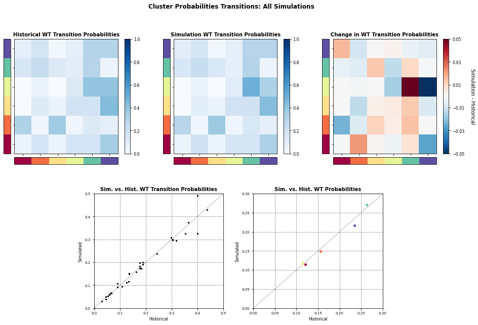
The chronological sequencing of AWTs was found significant to a second-order Markov chain, and simulated synthetic time series from the Markov chain reproduced not only the total probability and transition probabilities but also the average occurrence interval and persistence of each ENSO state. See the autoregressive logistic regression section below.
# --------------------------------------
# PCs123 random generation with Copulas

bmus = SST_AWTs.bmus.values[:]
PCs  = SST_AWTs.PCs.values[:]
vari = SST_AWTs.variance.values[:]

# first 3 PCs
PC1 = np.divide(PCs[:,0], np.sqrt(vari[0]))
PC2 = np.divide(PCs[:,1], np.sqrt(vari[1]))
PC3 = np.divide(PCs[:,2], np.sqrt(vari[2]))

# for each AWT: generate copulas and simulate data
PCs_fit = {}
PCs_rnd = {}
for ic in range(num_clusters):

    # find all the best match units
    ind = np.where(bmus == ic)[:]

    # PCs for weather type
    PC123 = np.column_stack((PC1[ind], PC2[ind], PC3[ind]))

    # statistical simulate PCs using copulas with KDE (kernel density estimation)
    PC123_rnd = copula_simulation(PC123, kernels, num_PCs_rnd)

    # store data at dictionaries
    PCs_fit['{0}'.format(ic+1)] = PC123
    PCs_rnd['{0}'.format(ic+1)] = PC123_rnd

# store PCs used for fitting and simulated
with open(SST_dPCs_fit_file, 'wb') as f:
    pickle.dump(PCs_fit, f, protocol=pickle.HIGHEST_PROTOCOL)

with open(SST_dPCs_rnd_file, 'wb') as f:
    pickle.dump(PCs_rnd, f, protocol=pickle.HIGHEST_PROTOCOL)
# Plot Weather Type 3D PCs for fit and random generation data
Plot_PCs_Compare_3D(PCs_fit, PCs_rnd);
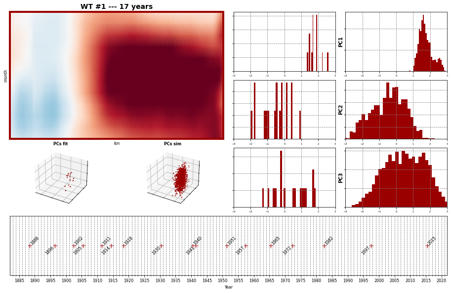
# Plot Annual Weather Types validation reports
Plot_AWTs_Validation(bmus, time, Km, num_clusters, lon, PCs_fit, PCs_rnd);
1.6. Autoregressive Logistic Regression#
The AWT sequence has been modeled by a second-order markov chain. Only the constant and mk_order parameters are active on the ALR settings, while the seasonality and long_term trend are deactivated.
Initially the model is fit, and a validation is performed at the end of the notebook.
In addition, categorical AWTs are converted to principal component space by defining tri-variate gaussian copulas (e.g. Wahl et al., 2012; Masina et al., 2015) for each AWT using the marginal distributions of its respective three PC components APC1, APC2, and APC3. Each simulated categorical ENSO is thus defined by a random number generator converted to a triplet of APC1, APC2, and APC3 from the appropriate copula, effectively providing synthetic time series with the potential to not only produce new chronologies, but also new SSTA behavior (i.e., create El Niño and La Niña events statistically consistent with observations but not exact replicas of the limited number of historical observations).
# --------------------------------------
# Autoregressive Logistic Regression - fit model

# bmus series
bmus_fit = xr.Dataset(
    {
        'bmus':(('time',), SST_AWTs.bmus.values[:] + 1),
    },
    coords = {'time': SST_AWTs.time.values[:]}
)

# ALR terms
d_terms_settings = {
    'mk_order'  : alr_markov_order,
    'constant' : True,
    'long_term' : False,
    'seasonality': (False, []),
}

# ALR wrapper
ALRW = ALR_WRP(alr_path)
ALRW.SetFitData(num_clusters, bmus_fit, d_terms_settings)

# ALR model fitting
ALRW.FitModel(max_iter=50000)
Fitting autoregressive logistic model ...
Optimization done in 0.09 seconds
# --------------------------------------
# Autoregressive Logistic Regression - simulate

# simulation dates (annual array)
dates_sim = [datetime(y, pca_month_ini,1) for y in range(y1_sim-1, y2_sim+1)]

# launch simulation
ALR_sim = ALRW.Simulate(num_sims, dates_sim)

# store simulated Annual Weather Types
SST_AWTs_sim = ALR_sim.evbmus_sims.to_dataset()

# save
save_nc(SST_AWTs_sim, sst_awt_sim_file, safe_time=True)
# show simulation report
ALRW.Report_Sim();
PerpetualYear bmus comparison skipped.
timedelta (days): Hist - 365, Sim - 366)
# --------------------------------------
# PCs generation

# solve each ALR simulation
l_PCs_sim = []
for s in SST_AWTs_sim.n_sim:

    evbmus_sim = SST_AWTs_sim.sel(n_sim=s).evbmus_sims.values[:]

    # generate random PCs
    pcs123_sim = np.empty((len(evbmus_sim),3)) * np.nan
    for c, m in enumerate(evbmus_sim):
        options = PCs_rnd['{0}'.format(int(m))]
        r = np.random.randint(options.shape[0])
        pcs123_sim[c,:] = options[r,:]

    # denormalize simulated PCs
    PC1_sim = np.multiply(pcs123_sim[:,0], np.sqrt(vari[0]))
    PC2_sim = np.multiply(pcs123_sim[:,1], np.sqrt(vari[1]))
    PC3_sim = np.multiply(pcs123_sim[:,2], np.sqrt(vari[2]))

    # append simulated PCs
    l_PCs_sim.append(
        xr.Dataset(
            {
                'PC1'  : (('time',), PC1_sim),
                'PC2'  : (('time',), PC2_sim),
                'PC3'  : (('time',), PC3_sim),
                'evbmus_sim' : (('time',), evbmus_sim),
            },
            {'time' : dates_sim}
        )
    )

# concatenate simulations
SST_PCs_sim = xr.concat(l_PCs_sim, 'n_sim')


# store yearly simulated PCs
save_nc(SST_PCs_sim, pcs_sim_file, safe_time=True)

# resample to daily and store
xds_d = xds_reindex_daily(SST_PCs_sim)
save_nc(xds_d, pcs_sim_d_file, safe_time=True)

# resample to monthly and store
xds_m = xds_reindex_monthly(SST_PCs_sim)
save_nc(xds_m, pcs_sim_m_file, safe_time=True)