Historical Daily Weather Types
Contents
7. Historical Daily Weather Types#
Obtain daily predictor (Daily Weather Types, DWTs) based on SLP & GradSLP and associated wave conditions to each DWT
inputs required:
ESTELA fields for the site location
SLP fields and gradients from CFS reanalysis
Historical Seas and swells (snakes)
Historical TCs inside radio 14
in this notebook:
Construct daily SLP+GradSLP predictor
Obtain Daily Weather Types (DWT)
Associate wave conditions to each DWT
Workflow:
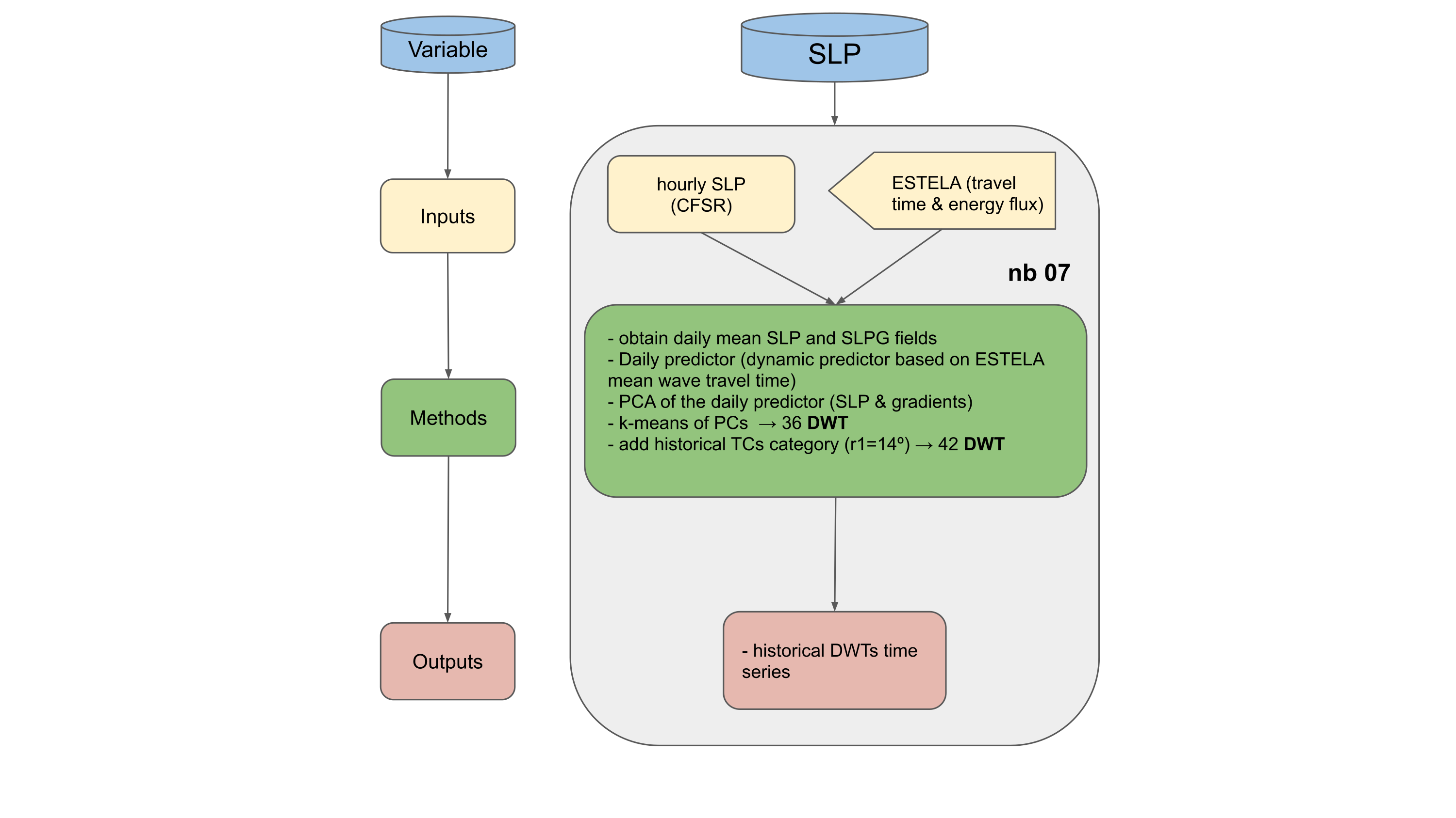
Daily SLP predictor:
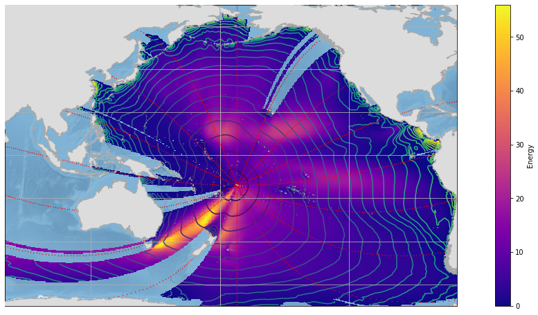
Weather is represented by sea level pressure (SLP) fields and the squared gradients (SLPG) of those fields obtained from the Climate Forecast System Reanalysis (CFSR) (Saha, et al., 2011). SLP fields effectively capture high- and low-pressure systems while SLPG are related to the strength of the wind stress generating waves and wind induced storm surge. Only the SLPs and SLPGs in a region considered to influence the site study are included in the analysis, however the size of the region extends to include distant weather systems due to the generation of swell which propagates across the ocean and affects the local wave runup. The region of influence was defined using the ESTELA(Evaluation of Source and Travel-time of wave Energy reaching a Local Area) method (Perez et al., 2014), which identifies the relevant amount of energy directed along great circle arcs toward the study site using full directional wave spectra in the global IFREMER wave hindcast (Rascle & Ardhuin, 2013). The SLP and SLPG fields were further modified to consider the travel time of swell waves, which arrive to the study site on the order of days to weeks after generation by a distant weather system. An atmospheric predictor, \(P_t\) , was created dependent on the isochrones of average wave travel time identified by ESTELA: \(P_t = \{...,{SLP}_{t-i+1,\Omega i},{SLPG}_{t-i+1,\Omega i}...\}\) for \(i =1,...,p\); where \(\Omega_i\) represents the spatial domain between the daily isochrones \(i - 1\) and \(\textit{i}\), and \(\textit{p}\) is the number of days of the last isochrone predicted by ESTELA, which represents the longest possible wave propagation time from generation until arrival at the target location.
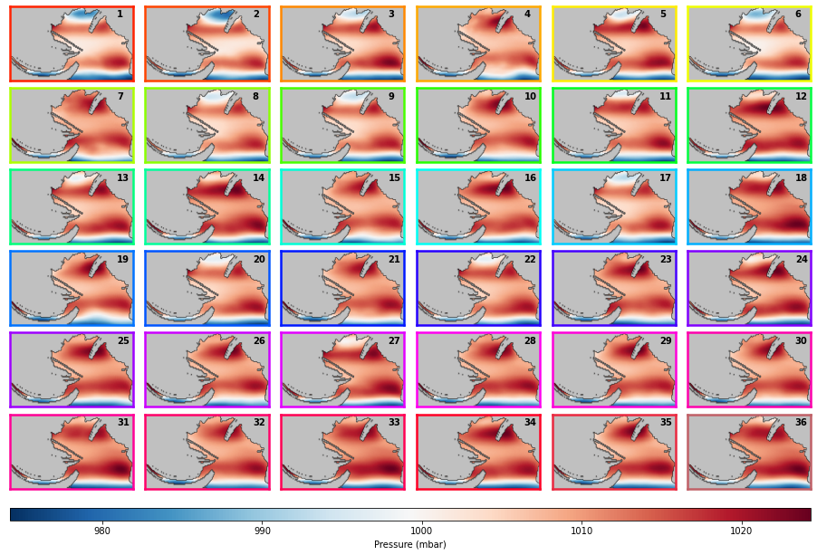
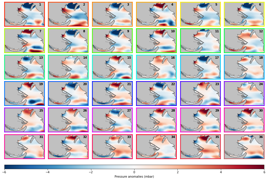
Weather-typing of the PCs of P_(t,x,y) was performed at a daily time scale to create a daily weather type (DWT) as a proxy for synoptic SLP patterns (Camus et al., 2014a, Camus et al. 2016). The number of clusters in this analysis was set at 36, and the regression guided K-means was performed iteratively until every cluster contained at least 50 days. Remapping the centroids of each cluster from PC space to SLP space results in the original DWT (figures below). Six additional DWTs were created to represent tropical depressions and tropical cyclone (TC) categories 1 through 5 by removing days with TC generation from the K-means clusters (ESTELA Predictor - Add Historical TCs) (TC generation defined in notebook 05). Separating the TCs as explicit categorical variables ensured that the probabilities of occurrence and conditional dependencies of the rare events were persevered in the framework rather than being clustered into extra-tropical synoptic circulation patterns as the most distance points from a prescribed centroid.
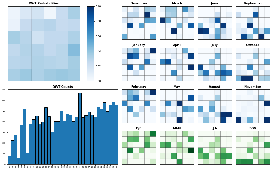
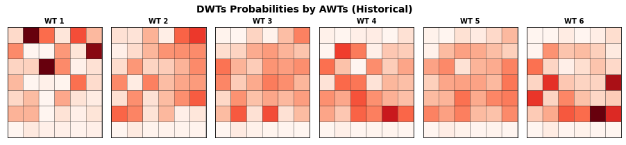
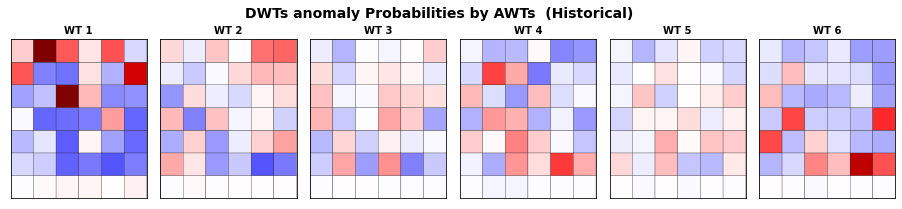
The 42 DWTs are presented in the figures below (ESTELA Predictor - KMeans Classification) as a matrix analogous to a self-organized map (Sheridan & Lee, 2011) to ensure that DWTs with similar spatial patterns are graphically presented adjacent to each other. Plot DWTs Probabilities and DWTs probabilities conditioned to IWT and AWT demonstrate how DWTs have historically exhibited conditional dependencies on the state of large-scale climate phenomena. The most readily discernable conditional dependencies are on seasonal scales where most DWTs exhibit a high probability of occurrence during a particular season and zero chance of occurring at other times. Although DWT dependencies on IWTs and AWTs are not as stark, probabilities of daily weather are still clearly affected, most notably with difference between the extremes of El Nino/La Nina and when the MJO is located on opposite sides of the globe.
Daily predictand:
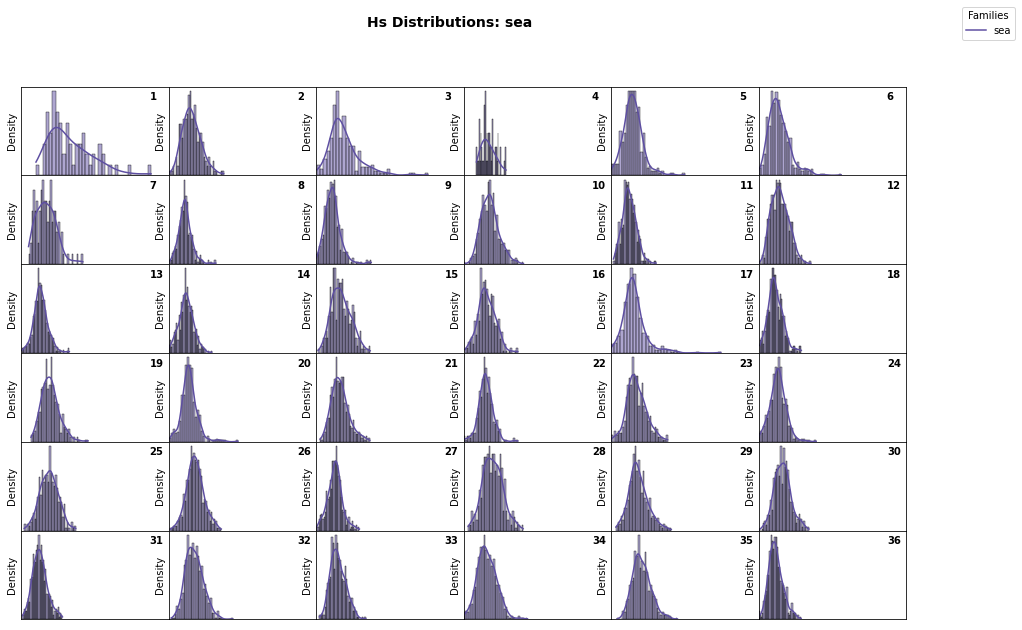
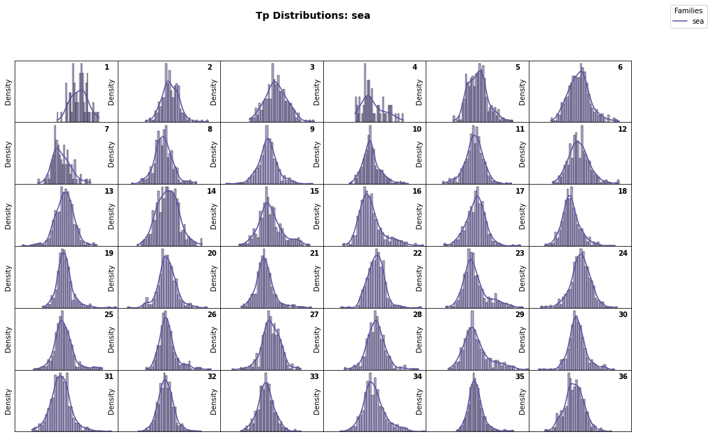
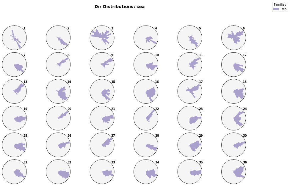
The DWT’s associated sea-state parameter distributions is provided at the end of the notebook to confirm how the automated identification of atmospheric variability also delineated variability within the local TWL components. The distributions of the three wave systems identified in notebook 09 conditioned to each DWT are shown.
#!/usr/bin/env python
# -*- coding: utf-8 -*-

# common
import os
import os.path as op

# pip
import numpy as np
import xarray as xr
from scipy.stats import circmean

import matplotlib.pyplot as plt

# DEV: override installed teslakit
import sys
sys.path.insert(0, op.join(os.path.abspath(''), '..', '..', '..', '..'))

# teslakit
from bluemath.teslakit2.wts.estela import dynamic_estela_predictor, Plot_PCs_3D, Mod_KMA_AddStorms
from bluemath.teslakit2.waves.snakes import add_bmus, group_by_dwt_dir_t
from bluemath.teslakit2.toolkit.pca import PCA_EstelaPred_slp_grd
from bluemath.teslakit2.toolkit.kma import slp_kmeans_clustering
from bluemath.teslakit2.util.time_operations import xds_common_dates_daily, xds_reindex_daily

from bluemath.teslakit2.plotting.estela import Plot_Estela, Plot_EOFs_EstelaPred, Plot_DWTs_Mean_Anom, Plot_DWTs_Probs
from bluemath.teslakit2.plotting.wts import Plot_Probs_WT_WT, Plot_Probs_WT_WT_anomaly
from bluemath.teslakit2.plotting.pcs import Plot_PCs_WT
from bluemath.teslakit2.plotting.snakes import plot_snakes_params
from bluemath.teslakit2.plotting.waves import Plot_Waves_DWTs
Warning: ecCodes 2.21.0 or higher is recommended. You are running version 2.20.0
7.1. Files and paths#
# project path
p_data =  r'/media/administrador/HD2/SamoaTonga/data'
site = 'Samoa'
p_site = op.join(p_data, site)

# deliverable folder
p_deliv = op.join(p_site, 'd09_TESLA')

# output path
p_out = op.join(p_deliv,'ESTELA')
if not os.path.isdir(p_out): os.makedirs(p_out)


# input data
estela_file = op.join(p_deliv,'resources','Estela_Samoa.nc')
tcs_hist_r1_params_file = op.join(p_deliv, 'TCs','TCs_hist_r1_params_samoa.nc') # TCs parameters r1
mjo_hist_file = op.join(p_deliv,'resources','MJO_hist.nc') # for plotting
sst_awt_file = op.join(p_deliv,'SST','SST_KMA.nc') # for plotting
snakes_file = op.join(p_deliv,'WAVES','Snakes_Parameters.nc') # for plotting
partitions_file = op.join(p_deliv,'WAVES','partitions_stats_wcut_1e-11.nc') # for plotting
slp_hist_file = op.join(p_deliv,'resources','SLP_hind_daily_wgrad.nc')


# output data
predictor_path = op.join(p_out,'pred_slp_grd') # path to store daily predictor results
if not os.path.isdir(predictor_path): os.makedirs(predictor_path)

data_file = op.join(predictor_path,'data.nc')
pca_file = op.join(predictor_path,'pca.nc')
kma_file = op.join(predictor_path,'kma.nc')

snakes_dwt_file = op.join(p_deliv,'WAVES','Snakes_Parameters_dwt.nc')
sea_dwt_file = op.join(p_deliv,'WAVES','Sea_partition_dwt.nc')
7.2. Parameters#
# --------------------------------------
# load data and set parameters

ESTELA = xr.open_dataset(estela_file,decode_times=False)           # ESTELA D data
SLP = xr.open_dataset(slp_hist_file)              # Historical csiro waves point

TCs_r1_params = xr.open_dataset(tcs_hist_r1_params_file)   # TCs historical parameters inside 14º radius

snakes = xr.open_dataset(snakes_file)
partitions = xr.open_dataset(partitions_file)

# KMA REGRESSION GUIDED parameters
kma_date_ini = '1979-01-01'
kma_date_end = '2021-01-01'
num_clusters = 36
7.3. ESTELA Predictor - Sea Level Pressure and Gradient#
ESTELA = ESTELA.sel(time='ALL')
ESTELA = ESTELA.assign({'estela_mask':(('latitude','longitude'),np.where(ESTELA.F.values>0,1,np.nan))})


# --------------------------------------
# Plot ESTELA and wave point coordinates

extent = [80, 290, -70, 70]
Plot_Estela(ESTELA,extent, figsize=[20,8]);
# --------------------------------------
# select time window and obtain daily means

SLP_d = SLP.sel(time = slice(kma_date_ini, kma_date_end)).resample(time='1D').mean()
SLP_d.to_netcdf(op.join(predictor_path,'data.nc'))

#SLP_d = xr.open_dataset(op.join(predictor_path,'data.nc'))
7.4. ESTELA Predictor - Principal Component Analysis#
# select ESTELA at site grid
ESTELA_site = ESTELA.sortby(ESTELA.latitude,ascending=False).interp(coords={'latitude':SLP_d.latitude,'longitude':SLP_d.longitude})

# apply ESTELA mask to SLP data
SLP_d['slp'] = SLP_d.slp * ESTELA_site.estela_mask
SLP_d['slp_gradient'] = SLP_d.slp_gradient * ESTELA_site.estela_mask
SLP_d['mask_land'] = ESTELA_site.estela_mask
# --------------------------------------
# Calculate ESTELA PCA

# generate estela predictor
estela_D = ESTELA_site.drop('time').traveltime
xds_estela_pred = dynamic_estela_predictor(SLP_d, 'slp', estela_D)

# calculate PCA
PCA = PCA_EstelaPred_slp_grd(xds_estela_pred, 'slp')

# save
PCA.to_netcdf(pca_file)

#PCA = xr.open_dataset(pca_file)
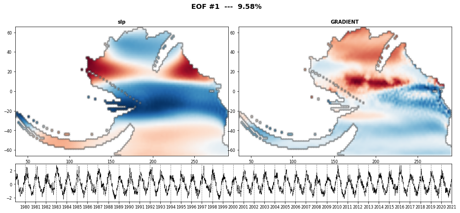
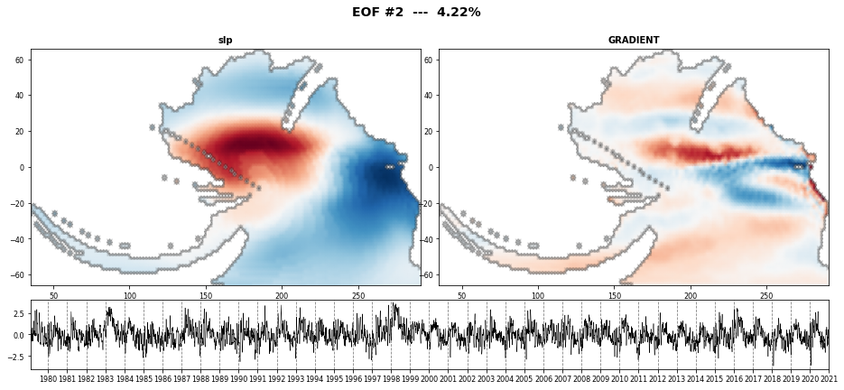
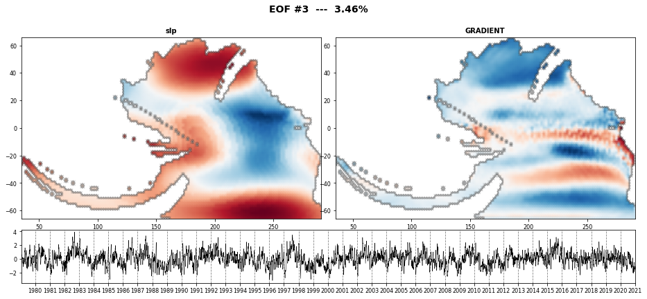
# plot PCA EOFs
n_EOFs = 3
vmin=-2
vmax=2

Plot_EOFs_EstelaPred(PCA, n_EOFs, show=True);
7.5. ESTELA Predictor - KMeans Classification#
# Calculate KMA (simple regression)

KMA = slp_kmeans_clustering(PCA, repres=0.95, num_clusters=num_clusters, min_data=50)

KMA['time']=(('n_components'), PCA.pred_time)

# float to int
KMA['sorted_bmus'].values = KMA['sorted_bmus'].values.astype(np.int32)

# save
KMA.to_netcdf(kma_file)

#KMA = xr.open_dataset(kma_file)
Number of PCs: 7830
Number of PCs explaining 95.0% of the EV is: 888
Iteration: 1Number of sims: 53
Minimum number of data: 62
# Plot DWTs (data mean)
Plot_DWTs_Mean_Anom(KMA, SLP_d['slp'], mask_land = SLP_d['mask_land'].values[:], kind='mean');
# Plot DWTs (data anomalies)
Plot_DWTs_Mean_Anom(KMA, SLP_d['slp'], mask_land = SLP_d['mask_land'].values[:], kind='anom');
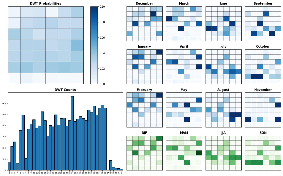
# Plot DWTs Probabilities

bmus = KMA['sorted_bmus'].values[:] + 1 # index to DWT id
bmus_time = KMA['time'].values[:]

Plot_DWTs_Probs(bmus, bmus_time, num_clusters, show=True);
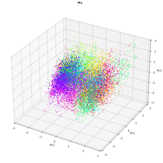
# Plot PC1, PC2, PC3 (3D)
Plot_PCs_3D(KMA, PCA);
# Plot PCs DWT centroids
# prepare data
PCs = PCA.PCs.values[:]
variance = PCA.variance.values[:]
bmus = KMA.sorted_bmus.values[:] # sorted_bmus
n_clusters = len(KMA.n_clusters.values[:])
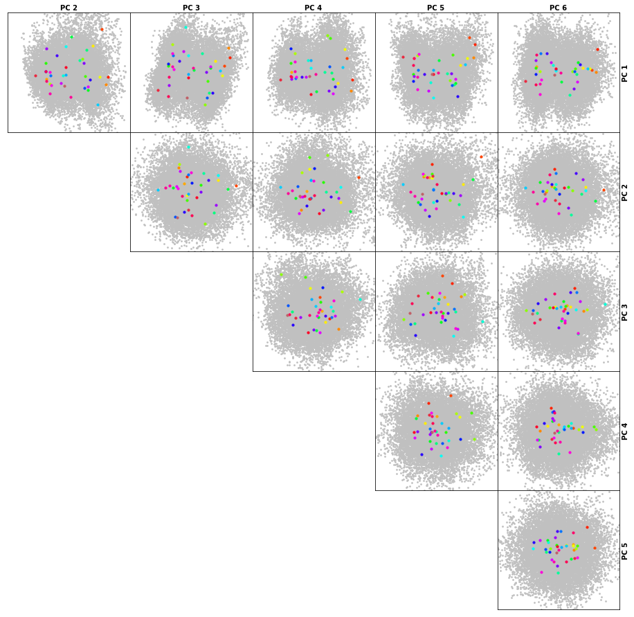
# Plot DWTs PCs
Plot_PCs_WT(PCs, variance, bmus, n_clusters, n=6);
7.6. ESTELA Predictor - Add Historical TCs#
# --------------------------------------
# use historical storms-parameters inside r1 to modify predictor KMA results

storm_dates = TCs_r1_params.dmin_date.values[:]
storm_categs = TCs_r1_params.category.values[:]

# add r1 storms to predictor KMA
KMA = Mod_KMA_AddStorms(KMA, storm_dates, storm_categs)

# save
if op.isfile(op.join(predictor_path,'kma.nc')): os.remove(op.join(predictor_path,'kma.nc'))
KMA.to_netcdf(op.join(predictor_path,'kma.nc'), mode ='w')
# Plot DWTs Probabilities with updated bmus

bmus = KMA['sorted_bmus_storms'].values[:] + 1 # index to DWT id
bmus_time = KMA['time'].values[:]

Plot_DWTs_Probs(bmus, bmus_time, 42, show=True);
# Plot MJO phases / DWTs Probabilities
#-------------------
# prepare data
MJO_hist = xr.open_dataset(mjo_hist_file)
# DWT historical - sorted_bmus
DWT_hist = xr.Dataset(
{'bmus': (('time',), KMA.sorted_bmus.values[:])},
coords = {'time': KMA.time.values[:]}
)
# get common dates
dc = xds_common_dates_daily([DWT_hist, MJO_hist])
DWT_hist = DWT_hist.sel(time=slice(dc[0], dc[-1]))
MJO_hist = MJO_hist.sel(time=slice(dc[0], dc[-1]))
#-------------------
# plot data
# num. MJO phases and DWTs
MJO_ncs = 8
DWT_ncs = 36
# categories to plot
MJO_phase = MJO_hist.phase.values[:] - 1
DWT_bmus = DWT_hist.bmus.values[:]
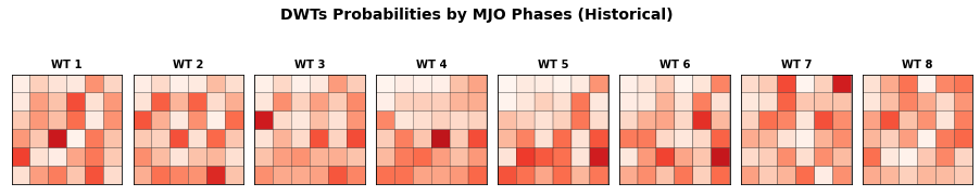
Plot_Probs_WT_WT(
MJO_phase, DWT_bmus, MJO_ncs, DWT_ncs,
wt_colors=False, ttl='DWTs Probabilities by MJO Phases (Historical)');
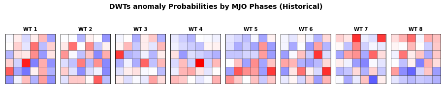
# plot DWTs conditional probabilities to each MJO, minus mean probabilities
Plot_Probs_WT_WT_anomaly(
MJO_phase, DWT_bmus, MJO_ncs, DWT_ncs,
wt_colors=False, ttl = 'DWTs anomaly Probabilities by MJO Phases (Historical)'
);
# Plot AWT / DWTs Probabilities

#-------------------
# prepare data

# AWTs historical data
xds_AWT = xr.open_dataset(sst_awt_file)

# AWT historical - bmus
xds_AWT = xr.Dataset(
    {'bmus': (('time',), xds_AWT.bmus.values[:])},
    coords = {'time': xds_AWT.time.values[:]}
)

# DWT historical - sorted_bmus_storms
xds_DWT = xr.Dataset(
    {'bmus': (('time',), KMA.sorted_bmus_storms.values[:])},
    coords = {'time': KMA.time.values[:]}
)

# reindex AWT to daily dates (year pad to days)
xds_AWT = xds_reindex_daily(xds_AWT)

# get common dates
dc = xds_common_dates_daily([xds_AWT, xds_DWT])
xds_DWT = xds_DWT.sel(time=slice(dc[0], dc[-1]))
xds_AWT = xds_AWT.sel(time=slice(dc[0], dc[-1]))


#-------------------
# plot data

# num. AWT phases and DWTs
AWT_ncs = 6
DWT_ncs = 42

# categories to plot
AWT_bmus = xds_AWT.bmus.values[:]
DWT_bmus =  xds_DWT.bmus.values[:]

Plot_Probs_WT_WT(
    AWT_bmus, DWT_bmus, AWT_ncs, DWT_ncs,
    wt_colors=False, ttl='DWTs Probabilities by AWTs (Historical)');


# plot DWTs conditional probabilities to each AWT, minus mean probabilities
Plot_Probs_WT_WT_anomaly(
    AWT_bmus, DWT_bmus, AWT_ncs, DWT_ncs,
    wt_colors=False, ttl = 'DWTs anomaly Probabilities by AWTs  (Historical)'
);
7.7. Wave conditions for each DWT#
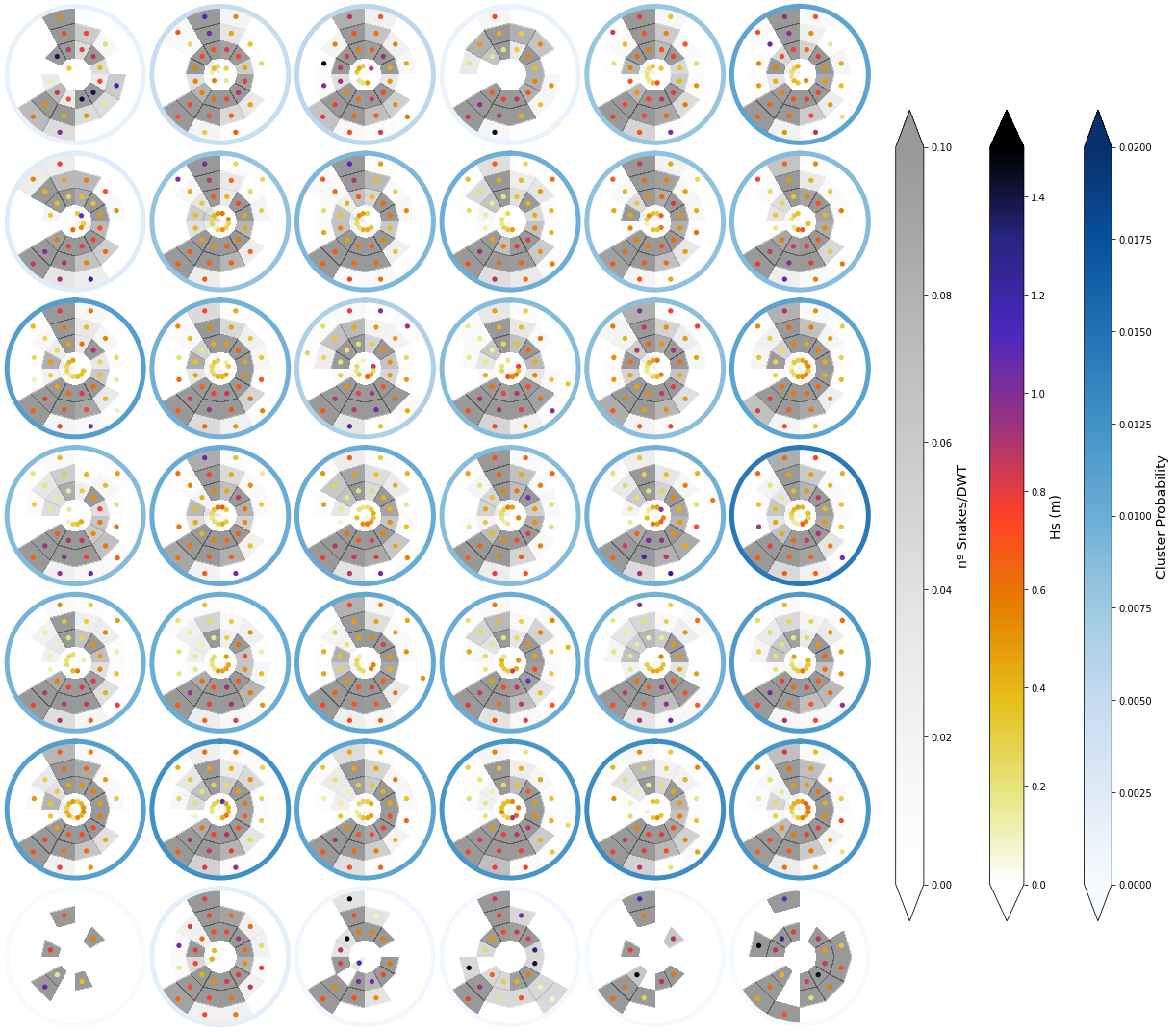
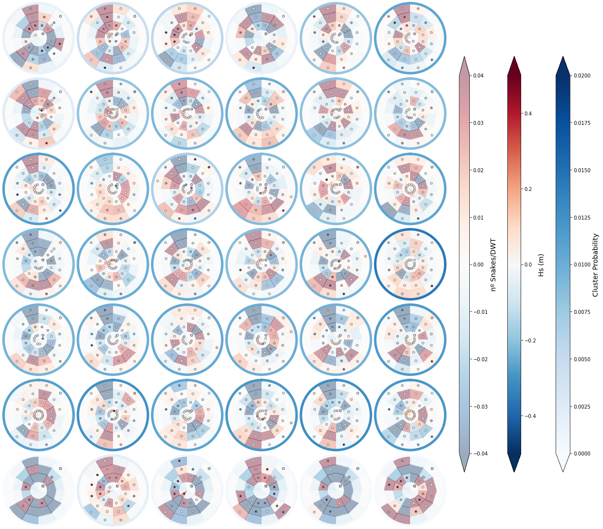
7.7.1. Swells (snakes ) parameters#
#------------------------------
# Swells (snakes) by DWTs

# select snakes for kma period
snakes=snakes.where(snakes.time>=KMA.time.values[0], drop=True)
snakes=snakes.where(snakes.time<=KMA.time.values[-1], drop=True)

# assign correspondent bmus to each snake
snakes = add_bmus(snakes, KMA)

# save
snakes.to_netcdf(snakes_dwt_file)


# Group snakes in each DWT by direction and period
n_dwts, n_snakes, hs_snakes = group_by_dwt_dir_t(snakes, KMA, n_clusters=42,amp_dir=30,amp_t=7,t_max=25)
# plot Swells (snakes) by DWTs

plot_snakes_params(n_dwts, n_snakes, hs_snakes,  amp_dir=30,amp_t=7,t_max=25, prob_max=0.06, vmax_z1=1.5)

plot_snakes_params(n_dwts, n_snakes, hs_snakes, annomaly=True, amp_dir=30,amp_t=7,t_max=25, prob_max=0.06, vmax_z1=.5)
7.7.2. Sea parameters#
#------------------------------
# Seas by DWTs

# select sea partition
sea_part = partitions.sel(part=0)

# select seas for kma period
sea_part=sea_part.where(sea_part.time>=KMA.time.values[0], drop=True)
sea_part=sea_part.where(sea_part.time<=KMA.time.values[-1], drop=True)

# obtain daily means
sea_part_d = sea_part.resample(time='D').mean()

sea_part_d['dir_mean'] = sea_part_d['dpm'].copy(deep=True)*np.nan
ind_d = 0
for d_ini, d_end in (zip(sea_part_d.time[:-1], sea_part_d.time[1:])):

    dir_d = sea_part.sel(time=slice(d_ini, d_end))
    dir_d = dir_d.dpm.isel(time=slice(0,-1)).values

    sea_part_d['dir_mean'][ind_d] = np.rad2deg(circmean(np.deg2rad(dir_d), nan_policy='omit'))

    ind_d = ind_d+1

sea_part_d = sea_part_d.drop({'dpm'})
sea_part_d = sea_part_d.rename({'dir_mean':'dpm'})

# add bmus to sea partition
sea_part_d = add_bmus(sea_part_d, KMA)

# save
sea_part_d.to_netcdf(sea_dwt_file)
# Plot Seas by DWTs

sea_part_d = sea_part_d[['hs', 'tp','dpm','bmus']]
sea_part_d = sea_part_d.rename({'hs':'sea_Hs', 'tp':'sea_Tp', 'dpm':'sea_Dir', })

n_clusters=36

Plot_Waves_DWTs(sea_part_d, sea_part_d.bmus.values, n_clusters);