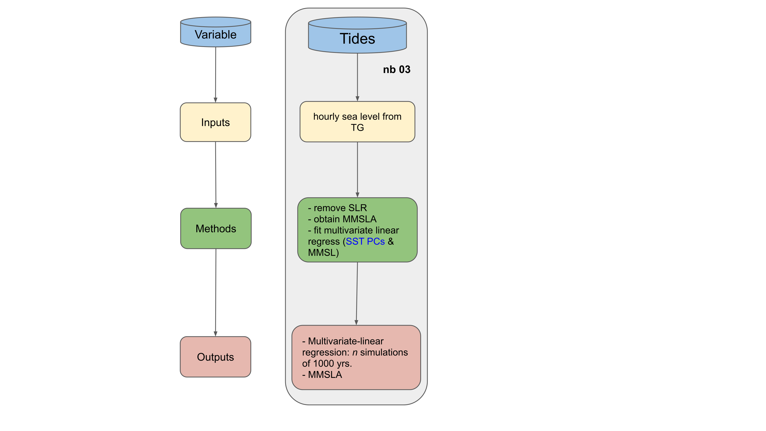
3. Monthly Mean Sea Level

Simulate Monthly Mean Sea Level (MMSL) using a multivariate-linear regression model based on the annual SST PCs

inputs required:

• WaterLevel historical data from a tide gauge at the study site

• Historical and simulated Annual PCs

in this notebook:

• Obtain monthly mean sea level anomalies (MMSLA) from the tidal gauge record

• Perform linear regression between MMSLA and annual PCs

• Obtain predicted timeseries of MMSLA based on simulated timeseries of annual PCs

Workflow:

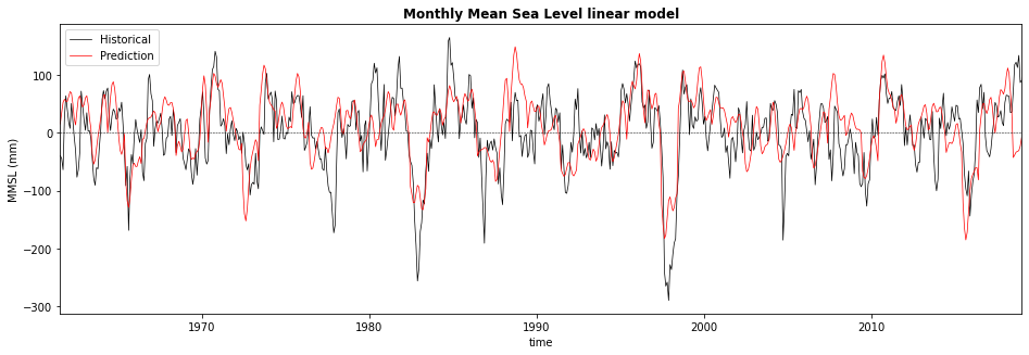
Monthly sea level variability is typically due to processes occurring at longer timescales than the daily weather. Slowly varying seasonality and anomalies due to ENSO are retained in the climate emulator via the principle components (APC) used to develop the AWT. A multivariate regression model containing a mean plus annual and seasonal cycles at 12-month and 6-month periods for each APC covariate was fit to the MMSLA. This simple model explains ~75% of the variance without any specific information regarding local conditions (i.e., local anomalies due to coastal shelf dynamics, or local SSTAs) and slightly underpredicts extreme monthly sea level anomalies by ~10 cm. While this component of the approach is a subject of ongoing research, the regression model produces an additional ~0.35 m of regional SWL variability about mean sea level, which was deemed sufficient for the purposes of demonstrating the development of the stochastic climate emulator.

#!/usr/bin/env python
# -*- coding: utf-8 -*-

# basic import
import os
import os.path as op

# python libs
import numpy as np
import pandas as pd
from numpy.random import multivariate_normal
import xarray as xr
from scipy.stats import linregress
from scipy.optimize import curve_fit

# DEV: override installed teslakit
import sys
sys.path.insert(0, op.join(os.path.abspath(''), '..','..', '..', '..'))

# teslakit
from bluemath.teslakit2.toolkit.averages import running_mean, monthly_mean
from bluemath.teslakit2.util.time_operations import date2yearfrac as d2yf
from bluemath.teslakit2.io.aux import save_nc

from bluemath.teslakit2.plotting.tides import Plot_Tide_SLR, Plot_Tide_RUNM, Plot_Tide_MMSL, \
Plot_Validate_MMSL_tseries, Plot_Validate_MMSL_scatter, Plot_MMSL_Prediction, \
Plot_MMSL_Histogram

Warning: ecCodes 2.21.0 or higher is recommended. You are running version 2.20.0

3.1. Files and paths

# project path
p_data =  r'/media/administrador/HD2/SamoaTonga/data'
site = 'Samoa'
p_site = op.join(p_data, site)

# deliverable folder
p_deliv = op.join(p_site, 'd09_TESLA')

# output path 
p_out = op.join(p_deliv,'TIDE')
if not os.path.isdir(p_out): os.makedirs(p_out)

    
# input data
TG_file = op.join(p_out,'tide_astro_hist_h056a.nc')
sst_awt_file = op.join(p_deliv,'SST','SST_KMA.nc') # KMA results
pcs_sim_m_file = op.join(p_deliv,'SST','SST_PCs_sim_m.nc') # PCs resampled to monthly

# output data
mmsl_hist_file = op.join(p_out,'tide_mmsl_hist.nc') # historical mmsl from TG
mmsl_sim_file = op.join(p_out,'tide_mmsl_sim.nc') # simulated mmsl from PCs
model_coefs_file = op.join(p_out,'mmsl_model_params.nc') # fitting parameters of the regression model

3.2. Parameters

# --------------------------------------
# load data and set parameters

WL_split = xr.open_dataset(TG_file)  # water level historical data (tide gauge)uge)
WL = WL_split.WaterLevels

SST_KMA = xr.open_dataset(sst_awt_file)             # SST Anual Weather Types PCs
SST_PCs_sim_m = xr.open_dataset(pcs_sim_m_file, decode_times=True)   # simulated SST PCs (monthly)

# parameters for mmsl calculation
mmsl_year_ini = 1947
mmsl_year_end = 2018

3.3. Monthly Mean Sea Level

# --------------------------------------
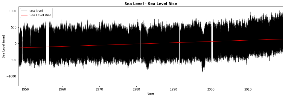
# Calculate SLR using linear regression

WL['time'] = WL['time'].dt.round('H')

time = WL.time.values[:]
wl = WL.values[:] * 1000  # (m to mm)

# MOVE TIME SERIES HALF A YEAR BACK
time = time - pd.Timedelta(days=366/2)

lr_time = np.array(range(len(time)))  # for linregress
mask = ~np.isnan(wl)  # remove nans with mask

slope, intercept, r_value, p_value, std_err = linregress(lr_time[mask], wl[mask])
slr = intercept + slope * lr_time

# Plot tide with SLR
Plot_Tide_SLR(time, wl, slr);

# --------------------------------------
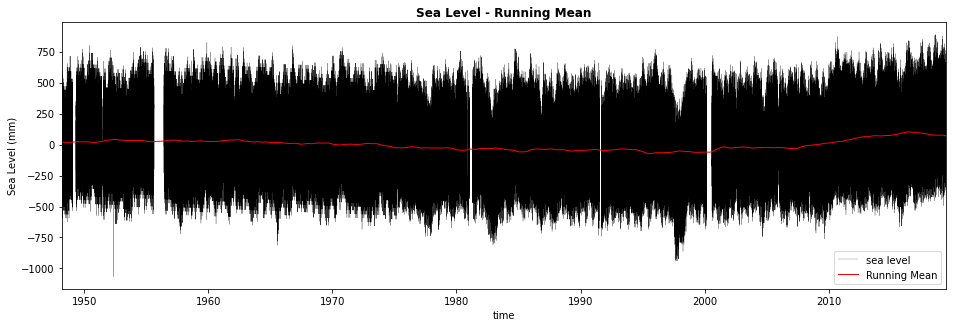
# remove SLR and runmean from tide 

tide_noslr = wl - slr

# calculate tide running mean
time_window = 365*24*3
runm = running_mean(tide_noslr, time_window, 'mean')

# remove running mean
tide_noslr_norunm = tide_noslr - runm

# store data 
TNSR = xr.DataArray(tide_noslr_norunm,  dims=('time'), coords={'time':time})


# Plot tide without SLR and runm
Plot_Tide_RUNM(time, tide_noslr, runm);

running_mean: input data contain NaNs!!

# --------------------------------------
# calculate Monthly Mean Sea Level (mmsl)

MMSL = monthly_mean(TNSR, mmsl_year_ini, mmsl_year_end)

# fill nans with interpolated values
p_nan = np.isnan(MMSL.data_mean)
MMSL.data_mean[p_nan]= np.interp(MMSL.time[p_nan], MMSL.time[~p_nan], MMSL.data_mean[~p_nan])

mmsl_time = MMSL.time.values[:]
mmsl_vals = MMSL.data_mean.values[:]

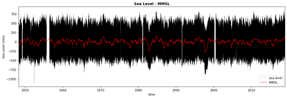
# Plot tide and mmsl 
Plot_Tide_MMSL(TNSR.time, TNSR.values, mmsl_time, mmsl_vals);

# store historical mmsl
save_nc(MMSL,mmsl_hist_file)

3.4. Monthly Mean Sea Level - Principal Components

The annual PCs are passed to a monthly resolution

# --------------------------------------
# SST Anual Weather Types PCs

PCs = np.array(SST_KMA.PCs.values)
PC1, PC2, PC3 = PCs[:,0], PCs[:,1], PCs[:,2]
PCs_years = [int(str(t).split('-')[0]) for t in SST_KMA.time.values[:]]

# MMSL PCs calculations: cut and pad it to monthly resolution
ntrs_m_mean = np.array([])
ntrs_time = []

MMSL_PC1 = np.array([])
MMSL_PC2 = np.array([])
MMSL_PC3 = np.array([])

for c, y in enumerate(PCs_years):
    pos = np.where(
        (mmsl_time >= np.datetime64('{0}-06-01'.format(y))) &
        (mmsl_time <= np.datetime64('{0}-05-29'.format(y+1)))
    )
    
    if pos[0].size:
        ntrs_m_mean = np.concatenate((ntrs_m_mean, mmsl_vals[pos]),axis=0)
        # TODO check for 0s and nans in ntrs_m_mean?
        ntrs_time.append(mmsl_time[pos])

        MMSL_PC1 = np.concatenate((MMSL_PC1, np.ones(pos[0].size)*PC1[c]),axis=0)
        MMSL_PC2 = np.concatenate((MMSL_PC2, np.ones(pos[0].size)*PC2[c]),axis=0)
        MMSL_PC3 = np.concatenate((MMSL_PC3, np.ones(pos[0].size)*PC3[c]),axis=0)

ntrs_time = np.concatenate(ntrs_time)

# Parse time to year fraction for linear-regression seasonality 
frac_year = np.array([d2yf(x) for x in ntrs_time])

3.5. Monthly Mean Sea Level - Multivariate-linear Regression Model

# --------------------------------------
# Fit linear regression model 

def modelfun(data, *x):
    pc1, pc2, pc3, t = data
    
    return x[0] + x[1]*pc1 + x[2]*pc2 + x[3]*pc3 + \
            np.array([x[4] + x[5]*pc1 + x[6]*pc2 + x[7]*pc3]).flatten() * np.cos(2*np.pi*t) + \
            np.array([x[8] + x[9]*pc1 + x[10]*pc2 + x[11]*pc3]).flatten() * np.sin(2*np.pi*t) + \
            np.array([x[12] + x[13]*pc1 + x[14]*pc2 + x[15]*pc3]).flatten() * np.cos(4*np.pi*t) + \
            np.array([x[16] + x[17]*pc1 + x[18]*pc2 + x[19]*pc3]).flatten() * np.sin(4*np.pi*t) 

# use non-linear least squares to fit our model
split = 160  # train / validation split index
x0 = np.ones(20)
sigma = np.ones(split)

# select data for scipy.optimize.curve_fit
x_train = ([MMSL_PC1[:split], MMSL_PC2[:split], MMSL_PC3[:split], frac_year[:split]])
y_train = ntrs_m_mean[:split]

res_lsq, res_cov = curve_fit(modelfun, x_train, y_train, x0, sigma)

3.6. Train and test model

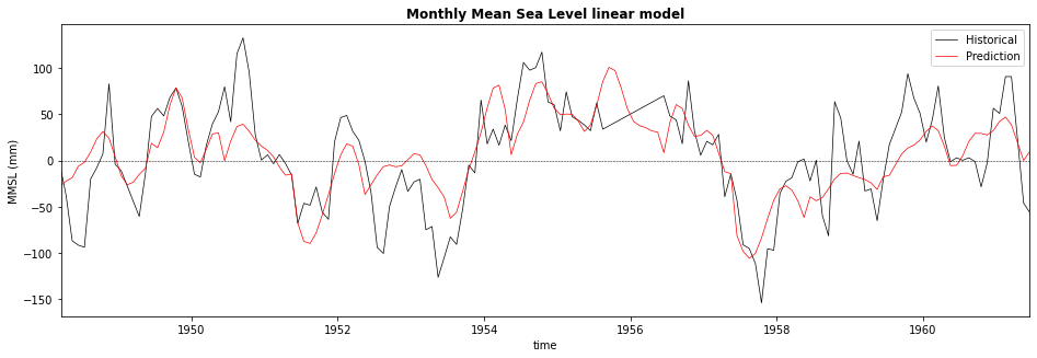
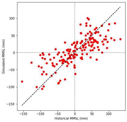
# Check model at fitting period

yp_train = modelfun(x_train, *res_lsq)

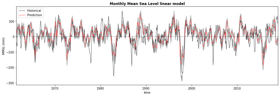
Plot_Validate_MMSL_tseries(ntrs_time[:split], ntrs_m_mean[:split], yp_train);
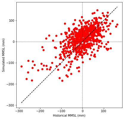
Plot_Validate_MMSL_scatter(ntrs_m_mean[:split], yp_train);

# Check model at validation period

x_val = ([MMSL_PC1[split:], MMSL_PC2[split:], MMSL_PC3[split:], frac_year[split:]])
yp_val = modelfun(x_val, *res_lsq)

Plot_Validate_MMSL_tseries(ntrs_time[split:], ntrs_m_mean[split:], yp_val);
Plot_Validate_MMSL_scatter(ntrs_m_mean[split:], yp_val);

# Parameter sampling (generate sample of params based on covariance matrix)

n_sims = 10
theta_gen = res_lsq
theta_sim = multivariate_normal(theta_gen, res_cov, n_sims)

# Check model at validation period
yp_valp = np.ndarray((n_sims, len(ntrs_time[split:]))) * np.nan
for i in range(n_sims):
    yp_valp[i, :] = modelfun(x_val, *theta_sim[i,:])

# 95% percentile
yp_val_quant = np.percentile(yp_valp, [2.275, 97.275], axis=0)

Plot_Validate_MMSL_tseries(ntrs_time[split:], ntrs_m_mean[split:], yp_val, mmsl_pred_quantiles=yp_val_quant);

# Fit model using entire dataset

sigma = np.ones(len(frac_year))
x_fit = ([MMSL_PC1, MMSL_PC2, MMSL_PC3, frac_year])
y_fit = ntrs_m_mean

res_lsq, res_cov = curve_fit(modelfun, x_fit, y_fit, x0, sigma)

# obtain model output
yp = modelfun(x_fit, *res_lsq)


# Generate 1000 simulations of the parameters 
n_sims = 1000
theta_gen = res_lsq
param_sim = multivariate_normal(theta_gen, res_cov, n_sims)


# Check model
yp_p = np.ndarray((n_sims, len(ntrs_time))) * np.nan
for i in range(n_sims):
    yp_p[i, :] = modelfun(x_fit, *param_sim[i,:])

# 95% percentile
yp_quant = np.percentile(yp_p, [2.275, 97.275], axis=0)

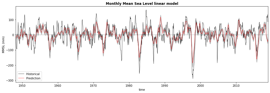
Plot_Validate_MMSL_tseries(ntrs_time, ntrs_m_mean, yp, mmsl_pred_quantiles=yp_quant);

# Save model parameters to use in climate change 
model_coefs = xr.Dataset({'sim_params' : (('n_sims','n_params'), param_sim)})
save_nc(model_coefs, model_coefs_file) 

3.7. Monthly Mean Sea Level - Prediction

# --------------------------------------
# Predict 1000 years using simulated PCs (monthly time resolution)

# get simulation time as year fractions
PCs_sim_time = SST_PCs_sim_m.time.values[:]
frac_year_sim = np.array([d2yf(x) for x in PCs_sim_time])

# solve each PCs simulation
y_sim_n = np.ndarray((len(SST_PCs_sim_m.n_sim), len(frac_year_sim))) * np.nan
for s in SST_PCs_sim_m.n_sim:
    
    PCs_s_m = SST_PCs_sim_m.sel(n_sim=s)
    MMSL_PC1_sim = PCs_s_m.PC1.values[:]
    MMSL_PC2_sim = PCs_s_m.PC2.values[:]
    MMSL_PC3_sim = PCs_s_m.PC3.values[:]
    
    # use linear-regression model
    x_sim = ([MMSL_PC1_sim, MMSL_PC2_sim, MMSL_PC3_sim, frac_year_sim])
    y_sim_n[s, :] = modelfun(x_sim, *param_sim[s,:])


# join output and store it
MMSL_sim = xr.Dataset(
    {
        'mmsl' : (('n_sim','time'), y_sim_n / 1000),  # mm to m
    },
    {'time' : PCs_sim_time}
)
print(MMSL_sim)

# save
save_nc(MMSL_sim, mmsl_sim_file, safe_time=True)

<xarray.Dataset>
Dimensions:  (n_sim: 100, time: 984)
Coordinates:
  * time     (time) datetime64[ns] 2019-06-01 2019-07-01 ... 2101-05-01
Dimensions without coordinates: n_sim
Data variables:
    mmsl     (n_sim, time) float64 0.01943 0.02091 0.03767 ... 0.07367 0.04747

# Plot mmsl simulation 

plot_sim = 0

y_sim = MMSL_sim.sel(n_sim=plot_sim).mmsl.values[:] * 1000  # m to mm
t_sim = MMSL_sim.sel(n_sim=plot_sim).time.values[:]

# Plot mmsl prediction
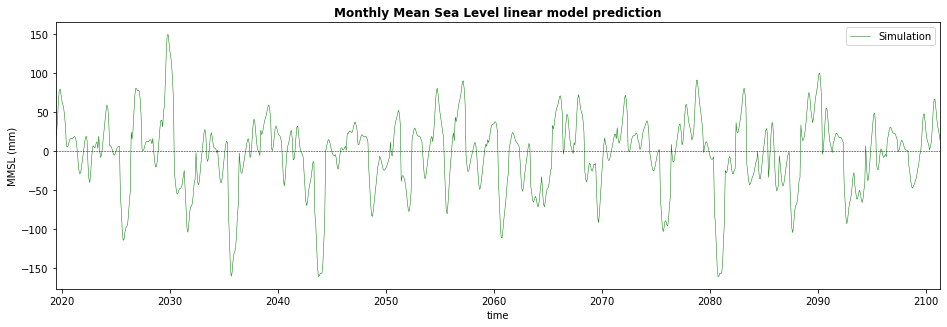
Plot_MMSL_Prediction(t_sim, y_sim);

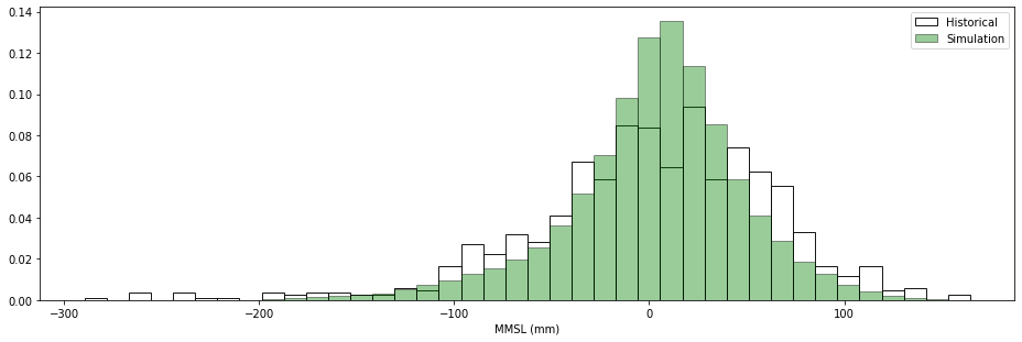
# compare model histograms
Plot_MMSL_Histogram(ntrs_m_mean, y_sim);

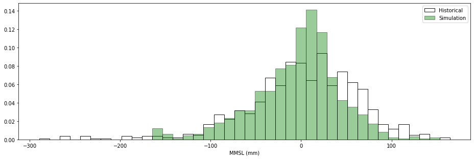
# compare model histograms for all simulations

y_sim = MMSL_sim.mmsl.values[:].flatten() * 1000  # m to mm

Plot_MMSL_Histogram(ntrs_m_mean, y_sim);