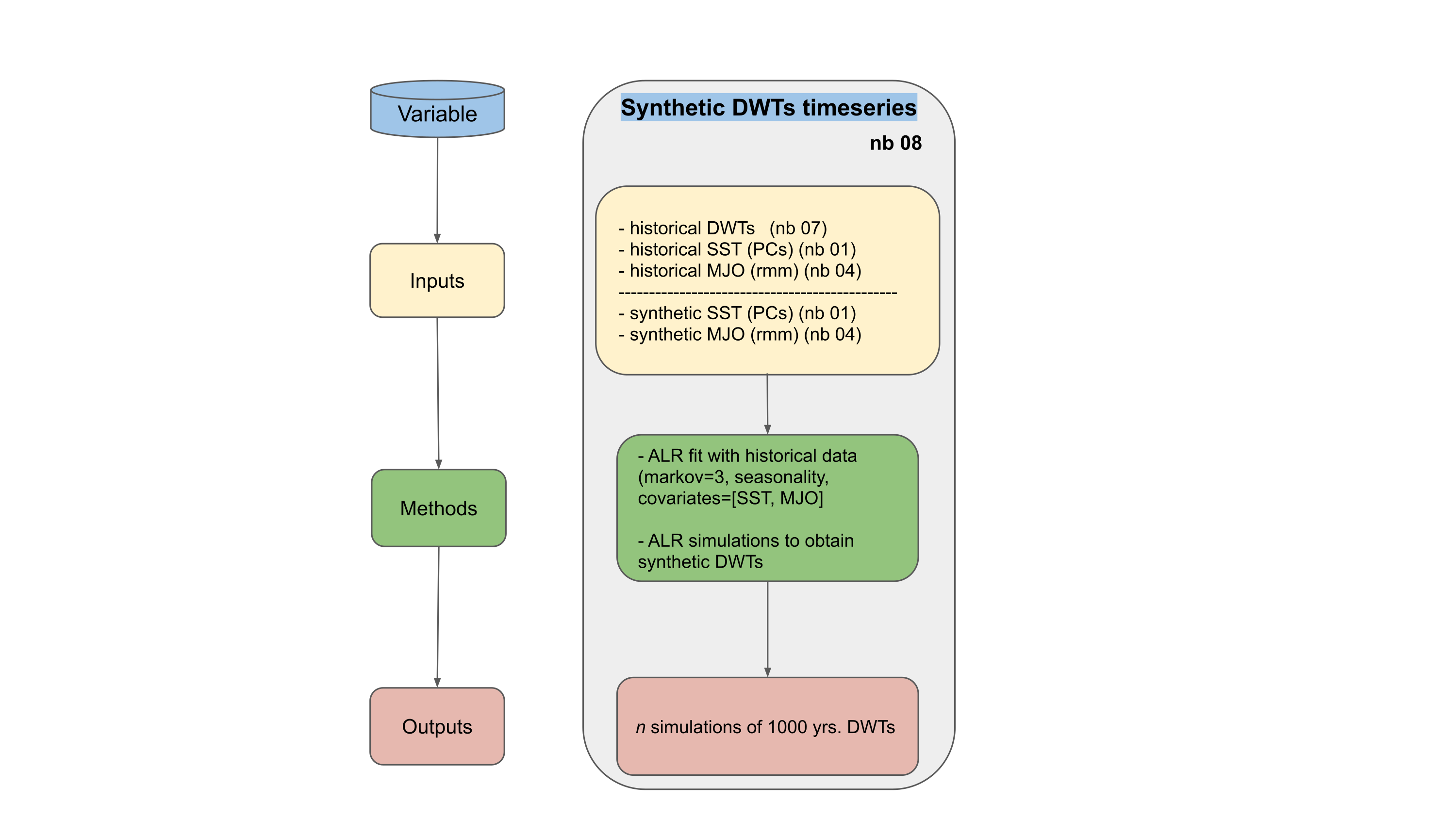
8. Synthetic Daily Weather Types

Obtain synthetic Daily Weather Types (DWTs) timeseries

inputs required:

• Historical DWTs

• Historical AWT and IWT

• Synthetic timeseries of AWT and IWT

in this notebook:

• Fit the ALR model of DWT based on seasonality, AWT and IWT timeseries

• Generate n simulations of 1000 years of DWTs timeseries

Workflow:

Simulating sequencing and persistence of synthetic DWTs is accomplished with an autoregressive logistic model (ALR). ALR models are simultaneously able to account for covariates varying at different timescales as well as the autocorrelation of those covariates at different orders (Guanche et al., 2013; Antolinez et al., 2015). In this sense, the AWT, seasonality, IWT, as well as the ordering (transitions between DWTs) and duration (persistence within a DWT) can all be accounted for within a single framework to make a categorical decision of what the weather pattern should be on any given day. Mathematically, the model is represented as:

            Prob\((Y_t=i|Y_{t-1},...,Y_{t-e},X_t)\) =

            \(= {{\exp{\large (}\beta_{0,i} + \beta_{1,i}\cos \omega t + \beta_{2,i}\sin \omega t + \sum\limits_{j=1}^{3}\beta_{j,i}^{awt} APC_j(t) + \sum\limits_{j=1}^{2}\beta_{j,i}^{iwt} IPC_j(t) + \sum\limits_{j=1}^e Y_{t-j\gamma j,i}{\large )}} \over {\sum\limits_{k=1}^{n_{DWT}} \exp{\large (}\beta_{0,k} + \beta_{1,k}\cos \omega t + \beta_{2,k}\sin \omega t + \sum\limits_{j=1}^{3}\beta_{j,k}^{awt} APC_j(t) + \sum\limits_{j=1}^{2}\beta_{j,k}^{iwt} IPC_j(t) + \sum\limits_{j=1}^e Y_{t-j\gamma j,k}{\large )}}}\);     

            \(\forall i = 1,...,n_{ss}\)

where \(\beta_{1,i}\) and \(\beta_{2,i}\) covariates account for the seasonal probabilites of each DWT. Covariates \(\beta_{j,k}^{awt} APC_j(t)\) account for each weather type’s probability associated with the leading three principle components used to create the AWTs, covariates \(\beta_{j,k}^{iwt} IPC_j(t)\) account for the leading two principle components of the MJO, and \(Y_{t-j}\) represents the DWT of the previous j-states, and \(\beta_{j,i}\) is the parameter associated with the previous j-state, and the order e corresponds to the number of previous states that influence the actual DWT. Each of these covariates was found to be statistically significant by the likelihood ratio (Guanche et al. 2014), where inclusion of a covariate required an improvement in prediction beyond a penalty associated with the added degrees of freedom. An iterative method began with the best univariate model (seasonality) and added each covariate in a pair-wise fashion to determine the next best model (seasonality + \(APC_1\)), continuing this process until all covariates were added.

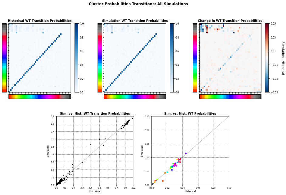
The model performance is evaluated at the end of the notebook by means of comparison historical and simulated probabilities of occurrence of the 42 DWTs during a perpetual year, the transition probabilities between DWTs and finally seasonal and conditional probabilities of occurrance of DWT to AWT and IWT.

#!/usr/bin/env python
# -*- coding: utf-8 -*-

# common
import os
import os.path as op

# pip
import numpy as np
import xarray as xr

import warnings
warnings.simplefilter(action='ignore')

# DEV: override installed teslakit
import sys
sys.path.insert(0, op.join(os.path.abspath(''), '..','..', '..', '..'))

# teslakit 
from bluemath.teslakit2.toolkit.alr import ALR_WRP
from bluemath.teslakit2.util.time_operations import xds_reindex_daily, xds_common_dates_daily
from bluemath.teslakit2.io.aux import save_nc

from bluemath.teslakit2.plotting.estela import Plot_DWTs_Probs
from bluemath.teslakit2.plotting.wts import Plot_Probs_WT_WT, Plot_Probs_WT_WT_anomaly

Warning: ecCodes 2.21.0 or higher is recommended. You are running version 2.20.0

8.1. Files and paths

# project path
p_data =  r'/media/administrador/HD2/SamoaTonga/data'
site = 'Samoa'
p_site = op.join(p_data, site)

# deliverable folder
p_deliv = op.join(p_site, 'd09_TESLA')

# output path 
p_out = op.join(p_deliv,'ESTELA')
if not os.path.isdir(p_out): os.makedirs(p_out)

    
# input data
alr_path = op.join(p_out,'alr_w') # path to store ALR results

mjo_hist_file = op.join(p_deliv,'resources','MJO_hist.nc')            # historical MJO
dwt_hist_file = op.join(p_deliv,'ESTELA','pred_slp_grd','kma.nc')   # ESTELA + TCs Predictor
awt_PCs_hist_file = op.join(p_deliv,'SST','SST_PCA.nc')               # SST PCs (annual)
awt_hist_file = op.join(p_deliv,'SST','SST_KMA.nc')               # for plotting

mjo_sim_file = op.join(p_deliv,'MJO','MJO_sim.nc')                    # MJO simulations (daily)
awt_PCs_sim_file = op.join(p_deliv,'SST','SST_PCs_sim_d.nc')          # SST PCs simulations (daily)
awt_sim_file = op.join(p_deliv,'SST','SST_AWT_sim.nc')                # SST PCs simulations (daily)

# output data
dwt_sim_file = op.join(p_out,'DWT_sim.nc')  

8.2. Parameters

# --------------------------------------
# load data and set parameters

MJO_fit = xr.open_dataset(mjo_hist_file)     # historical MJO
KMA_fit = xr.open_dataset(dwt_hist_file)     # ESTELA + TCs Predictor
PCs_all = xr.open_dataset(awt_PCs_hist_file)     # SST PCs (annual)

MJO_sim_all = xr.open_dataset(mjo_sim_file)     # MJO simulations (daily)
PCs_sim_all = xr.open_dataset(awt_PCs_sim_file)  # SST PCs simulations (daily)

# ALR fit parameters
alr_num_clusters = 42
alr_markov_order = 3
alr_seasonality = [2, 4, 6]

# ALR simulation
num_sims = 100  # one simulation for each simulated MJO, SST 

8.3. ESTELA Predictor - Autoregressive Logistic Regression Fitting

# --------------------------------------
# Data used to FIT ALR model and preprocess: 

# KMA: bmus (daily) (use sorted_bmus_storms, add 1 to get 1-42 bmus set)
BMUS_fit = xr.Dataset(
    {
        'bmus':(('time',), KMA_fit['sorted_bmus_storms'].values[:] + 1),
    },
    coords = {'time': KMA_fit.time.values[:]}
)


# SST: PCs (annual)
sst_PCs = PCs_all.PCs.values[:]
PCs_fit = xr.Dataset(
    {
        'PC1': (('time',), sst_PCs[:,0]),
        'PC2': (('time',), sst_PCs[:,1]),
        'PC3': (('time',), sst_PCs[:,2]),
    },
    coords = {'time': PCs_all.time.values[:]}
)

# reindex annual data to daily data
PCs_fit = xds_reindex_daily(PCs_fit)

# --------------------------------------
# Mount covariates matrix (model fit: BMUS_fit, MJO_fit, PCs_fit)

# covariates_fit dates
d_fit = xds_common_dates_daily([MJO_fit, PCs_fit, BMUS_fit])

# KMA dates
BMUS_fit = BMUS_fit.sel(time = slice(d_fit[0], d_fit[-1]))

# PCs covars 
cov_PCs = PCs_fit.sel(time = slice(d_fit[0], d_fit[-1]))
cov_1 = cov_PCs.PC1.values.reshape(-1,1)
cov_2 = cov_PCs.PC2.values.reshape(-1,1)
cov_3 = cov_PCs.PC3.values.reshape(-1,1)

# MJO covars
cov_MJO = MJO_fit.sel(time = slice(d_fit[0], d_fit[-1]))
cov_4 = cov_MJO.rmm1.values.reshape(-1,1)
cov_5 = cov_MJO.rmm2.values.reshape(-1,1)

# join covars 
cov_T = np.hstack((cov_1, cov_2, cov_3, cov_4, cov_5))

# normalize
cov_norm_fit = (cov_T - cov_T.mean(axis=0)) / cov_T.std(axis=0)
cov_fit = xr.Dataset(
    {
        'cov_norm': (('time','n_covariates'), cov_norm_fit),
        'cov_names': (('n_covariates',), ['PC1','PC2','PC3','MJO1','MJO2']),
    },
    coords = {'time': d_fit}
)

# --------------------------------------
# Autoregressive Logistic Regression

# model fit: BMUS_fit, cov_fit, num_clusters
# model sim: cov_sim, sim_num, sim_years

# ALR terms
d_terms_settings = {
    'mk_order'  : alr_markov_order,
    'constant' : True,
    'long_term' : False,
    'seasonality': (True, alr_seasonality),
    'covariates': (True, cov_fit),
}

# ALR wrapper
ALRW = ALR_WRP(alr_path)
ALRW.SetFitData(alr_num_clusters, BMUS_fit, d_terms_settings)

# ALR model fitting
ALRW.FitModel(max_iter=50000)

#ALRW.LoadModel()

Fitting autoregressive logistic model ...
Optimization done in 157.39 seconds

# Plot model p-values and params
ALRW.Report_Fit()

warning - statsmodels MNLogit could not provide p-values

8.4. ESTELA Predictor - Autoregressive Logistic Regression Simulation

# --------------------------------------
# Prepare Covariates for ALR simulations

# simulation dates
d_sim = xds_common_dates_daily([MJO_sim_all, PCs_sim_all])

# join covariates for all MJO, PCs simulations
l_cov_sims = []
for i in MJO_sim_all.n_sim: 

    # select simulation
    MJO_sim = MJO_sim_all.sel(n_sim=i)
    PCs_sim = PCs_sim_all.sel(n_sim=i)

    # PCs covar 
    cov_PCs = PCs_sim.sel(time = slice(d_sim[0], d_sim[-1]))
    cov_1 = cov_PCs.PC1.values.reshape(-1,1)
    cov_2 = cov_PCs.PC2.values.reshape(-1,1)
    cov_3 = cov_PCs.PC3.values.reshape(-1,1)

    # MJO covars
    cov_MJO = MJO_sim.sel(time = slice(d_sim[0], d_sim[-1]))
    cov_4 = cov_MJO.rmm1.values.reshape(-1,1)
    cov_5 = cov_MJO.rmm2.values.reshape(-1,1)

    # join covars (do not normalize simulation covariates)
    cov_T_sim = np.hstack((cov_1, cov_2, cov_3, cov_4, cov_5))
    cov_sim = xr.Dataset(
        {
            'cov_values': (('time','n_covariates'), cov_T_sim),
        },
        coords = {'time': d_sim}
    )
    l_cov_sims.append(cov_sim)

# use "n_sim" name to join covariates (ALR.Simulate() will recognize it)
cov_sims = xr.concat(l_cov_sims, dim='n_sim')
cov_sims = cov_sims.squeeze()

# --------------------------------------
# Autoregressive Logistic Regression - simulate 

# launch simulation
xds_alr = ALRW.Simulate(num_sims, d_sim, cov_sims, overfit_filter=True)

# Store Daily Weather Types
DWT_sim = xds_alr.evbmus_sims.to_dataset()
save_nc(DWT_sim, dwt_sim_file, True)

ALR model fit   : 1979-01-26 --- 2020-06-01
ALR model sim   : 2020-01-01 --- 2100-01-01

Launching 100 simulations...

# show sim report
ALRW.Report_Sim(py_month_ini=6, persistences_table=False);

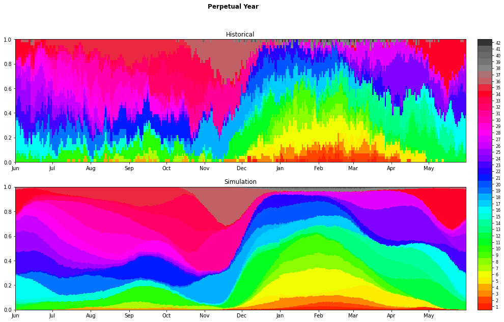
8.5. Compare historical and simulated DWTs probabilities

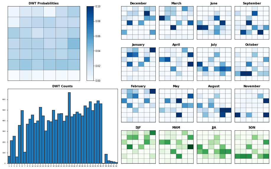
# Plot Historical DWTs probabilities (with TCs DWTs)

bmus_fit = KMA_fit.sorted_bmus_storms.values[:] + 1
dbmus_fit = KMA_fit.time.values[:]

Plot_DWTs_Probs(bmus_fit, dbmus_fit, alr_num_clusters);

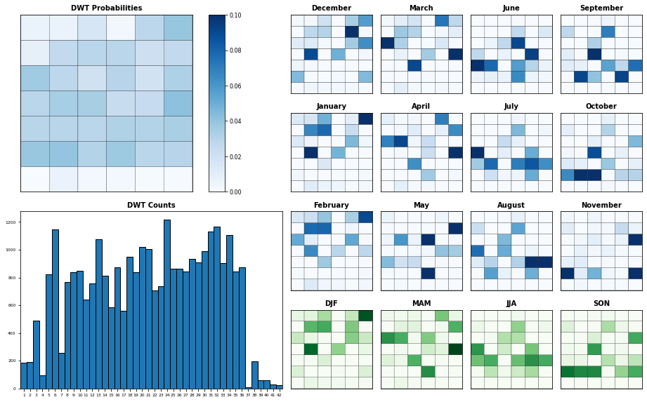
# Plot Simulated DWTs probabilities (with TCs DWTs)

bmus_sim = DWT_sim.isel(n_sim=0).evbmus_sims.values[:]
dbmus_sim = DWT_sim.time.values[:]

Plot_DWTs_Probs(bmus_sim, dbmus_sim, alr_num_clusters);

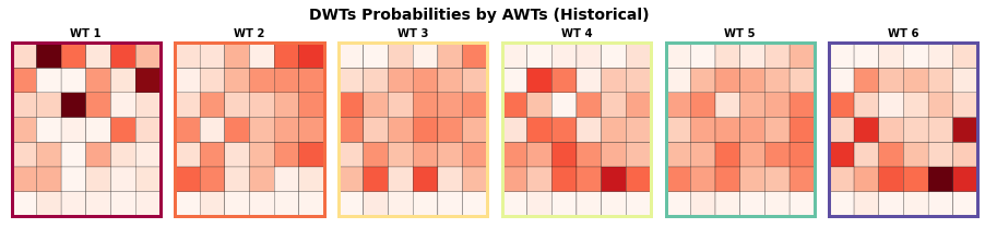
8.6. DWTs probabilities conditioned to AWTs

# Plot AWTs/DWTs Probabilities 

awt_his = xr.open_dataset(awt_hist_file)

# clusters to plot 
n_clusters_AWT = 6
n_clusters_DWT = 42
n_sim = 0  # simulation to plot


#--------------------------------
# Plot AWTs/DWTs Probs - historical

# AWTs historical data     
xds_AWT = xr.Dataset(
    {'bmus': (('time',), awt_his.bmus.values[:])},
    coords = {'time': awt_his.time.values[:]}
)

# DWT historical - sorted_bmus_storms
xds_DWT = xr.Dataset(
    {'bmus': (('time',), KMA_fit.sorted_bmus_storms.values[:])},
    coords = {'time': KMA_fit.time.values[:]}
)

# reindex AWT to daily dates (year pad to days)
xds_AWT = xds_reindex_daily(xds_AWT)

# get common dates
dc = xds_common_dates_daily([xds_AWT, xds_DWT])
xds_DWT = xds_DWT.sel(time=slice(dc[0], dc[-1]))
xds_AWT = xds_AWT.sel(time=slice(dc[0], dc[-1]))

# categories to plot
AWT_bmus_hist = xds_AWT.bmus.values[:]
DWT_bmus_hist =  xds_DWT.bmus.values[:]


Plot_Probs_WT_WT(
    AWT_bmus_hist, DWT_bmus_hist, n_clusters_AWT, n_clusters_DWT,
    wt_colors=True, ttl = 'DWTs Probabilities by AWTs (Historical)'
);


#--------------------------------
# Plot AWTs/DWTs sim - simulated

# simulated
xds_AWT = xr.open_dataset(awt_sim_file)


# AWT simulated - evbmus_sims -1 
xds_AWT = xr.Dataset(
    {'bmus': (('time',), xds_AWT.evbmus_sims.isel(n_sim=n_sim)-1)},
    coords = {'time': xds_AWT.time.values[:]}
)

# DWT simulated - evbmus_sims -1
xds_DWT = xr.Dataset(
    {'bmus': (('time',), DWT_sim.evbmus_sims.isel(n_sim=n_sim)-1)},
    coords = {'time': DWT_sim.time.values[:]}
)

# reindex AWT to daily dates (year pad to days)
xds_AWT = xds_reindex_daily(xds_AWT)

# get common dates
dc = xds_common_dates_daily([xds_AWT, xds_DWT])
xds_DWT = xds_DWT.sel(time=slice(dc[0], dc[-1]))
xds_AWT = xds_AWT.sel(time=slice(dc[0], dc[-1]))

AWT_bmus_sim = xds_AWT.bmus.values[:]
DWT_bmus_sim = xds_DWT.bmus.values[:]

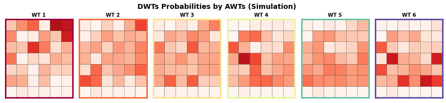
Plot_Probs_WT_WT(
    AWT_bmus_sim, DWT_bmus_sim, n_clusters_AWT, n_clusters_DWT,
    wt_colors=True, ttl = 'DWTs Probabilities by AWTs (Simulation)'
);

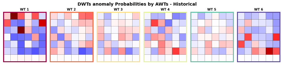
# plot DWTs conditional probabilities to each AWT, minus mean probabilities

# Plot AWTs/DWTs Probs - historical

Plot_Probs_WT_WT_anomaly(
    AWT_bmus_hist, DWT_bmus_hist, n_clusters_AWT, n_clusters_DWT,
    wt_colors=True, ttl = 'DWTs anomaly Probabilities by AWTs - Historical'
);


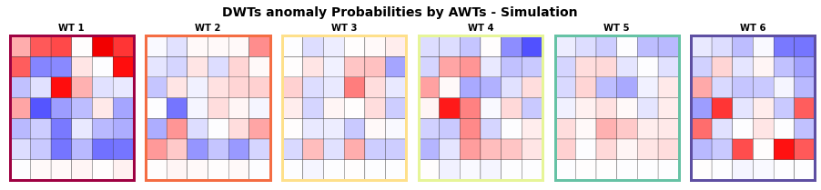
# Plot AWTs/DWTs sim - simulated

Plot_Probs_WT_WT_anomaly(
    AWT_bmus_sim, DWT_bmus_sim, n_clusters_AWT, n_clusters_DWT,
    wt_colors=True, ttl = 'DWTs anomaly Probabilities by AWTs - Simulation'
);