HyFlood

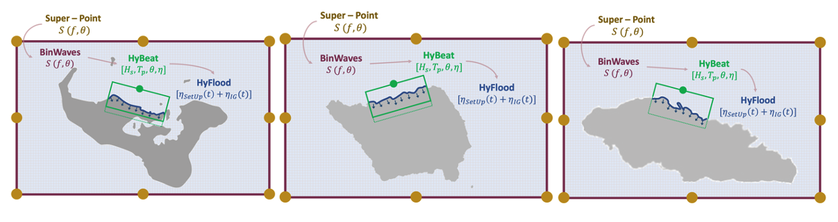
• HyFlood: This metamodel, based on a library of prerun cases of representative hyetographs using Lisflood-FP, allows to obtain the flooding maps as the convolution of flooding events every 500m of the coast.

This notebook alows to plot the flood map of a given Hypercube-sampled case, for a transect in a mesh.

Needed data:

• Flood cases in pickle format, all contained inside a folder.
  These are the outputs from Lisflood-FP runs, which contain a set of XYZ points, where Z is the maximum elevation obtained in that coordinate for the case.

• Digital Elevation Model (DEM) in NetCDF format.
  The name coding is as follows: “XL_N.nc” where X is the initial letter of the island and N is the mesh number. Therefore, “UL_04.nc” would be the fourth mesh of Upolu island.

• Synthetic events in NetCDF format.
  It contains a xarray.Dataset of 50 cases defined by their volume (V), their maximum level (Z*), their IG wave amplitude (Asig) and their duration (D). This cases are generated following the Latin Hypercube Sampling technique, which generates a random multidimensional set of parameters by arbitrary discretizing each dimension in N equally probable intervals.

• Shoreline in pickle format.
  It contains an array of float64 with X, Y and transect ID of every shoreline point of the selected site.

import os
import os.path as op
import sys

import numpy as np
import pandas as pd
import xarray as xr
import pickle
from natsort import natsorted

import matplotlib.pyplot as plt
import cmocean as cmo
import copy

from HyFlood_plots.plots import *
from ipywidgets import FloatProgress
from IPython.display import display
from time import sleep

Select location

Selection of the desired site. In this case there is only one possible island, Tongatapu.

It has 212 transects divided into 11 meshes.

The Highest Astronomical Tide in Tongatapu is 0.869m.

Parameters

Site : Desired island
Mesh : Mesh ID
Transect : Transect ID

#-----------------------------------------------------------
site     = 'tonga'    # ['tonga']
mesh     = 1         # Check the number of meshes of your island (above)   
transect = 50          # Check the transects for your island (above) 
#-----------------------------------------------------------

# Coordinate system and name code
code = 'T'
epsg = 32701 
hat  = 0.869          # Highest Astronomical Tide 

# INPUT PATHS
pdat = op.abspath(op.join(os.getcwd(), '..'))
pcas = op.join(pdat,'compressed_outputs_{0}L_{1:02d}'.format(code,mesh))
pdem = op.join(pdat,'data/sites/{0}/meshes'.format(site))
phyd = op.join(pdat,'data/sites/{0}/forcings'.format(site))
psho = op.join(pdat,'data/sites/{0}/shoreline'.format(site))

# OUTPUT PATHS
pfig = op.join(os.getcwd(),'figures/')
if not op.isdir(pfig):  os.makedirs(pfig)

# LOAD DATA
print('Island: {0} \t Mesh: {1}L_{2:02d} \t Transect: {3} \t \n'.format(site,code,mesh,transect))

# Floods
wds = []
for root, _, file in os.walk(pcas):   
    for name in file:
        if name.startswith('max_t{0:03d}'.format(transect)):
            wds.append(name)
            
wds = natsorted(wds)

print('Cases in the transect: {0} \n'.format(len(wds)))
print(wds)

# DEM
dem = xr.open_dataset(op.join(pdem,'{0}L_{1:02d}.nc'.format(code,mesh)))                 
# Forcings
hyd = xr.open_dataset(op.join(phyd,'cases50_IG.nc'))                                     
# Shoreline
sh  = pd.read_pickle(op.join(psho, 'shore_{0}_transects.pkl'.format(site)))              

Island: tonga 	 Mesh: TL_01 	 Transect: 50 	 

Cases in the transect: 50 

['max_t050_case00.pkl', 'max_t050_case01.pkl', 'max_t050_case02.pkl', 'max_t050_case03.pkl', 'max_t050_case04.pkl', 'max_t050_case05.pkl', 'max_t050_case06.pkl', 'max_t050_case07.pkl', 'max_t050_case08.pkl', 'max_t050_case09.pkl', 'max_t050_case10.pkl', 'max_t050_case11.pkl', 'max_t050_case12.pkl', 'max_t050_case13.pkl', 'max_t050_case14.pkl', 'max_t050_case15.pkl', 'max_t050_case16.pkl', 'max_t050_case17.pkl', 'max_t050_case18.pkl', 'max_t050_case19.pkl', 'max_t050_case20.pkl', 'max_t050_case21.pkl', 'max_t050_case22.pkl', 'max_t050_case23.pkl', 'max_t050_case24.pkl', 'max_t050_case25.pkl', 'max_t050_case26.pkl', 'max_t050_case27.pkl', 'max_t050_case28.pkl', 'max_t050_case29.pkl', 'max_t050_case30.pkl', 'max_t050_case31.pkl', 'max_t050_case32.pkl', 'max_t050_case33.pkl', 'max_t050_case34.pkl', 'max_t050_case35.pkl', 'max_t050_case36.pkl', 'max_t050_case37.pkl', 'max_t050_case38.pkl', 'max_t050_case39.pkl', 'max_t050_case40.pkl', 'max_t050_case41.pkl', 'max_t050_case42.pkl', 'max_t050_case43.pkl', 'max_t050_case44.pkl', 'max_t050_case45.pkl', 'max_t050_case46.pkl', 'max_t050_case47.pkl', 'max_t050_case48.pkl', 'max_t050_case49.pkl']

# PREPROCESS
# Mesh limits
#xmin, xmax = np.amin(dem.x.values), np.amax(dem.x.values)
#ymin, ymax = np.amin(dem.y.values), np.amax(dem.y.values)

# Nukualofa transect limits
xmin, xmax = [683000,688500]
ymin, ymax = [7657000,7662500]

# Cut shore
sx = np.where((sh[:,0] >= xmin) & (sh[:,0] <= xmax))[0]
sht = sh[sx]
sy = np.where((sht[:,1] >= ymin) & (sht[:,1] <= ymax))[0]
sht = sht[sy]

# Get transects inside the domain
transects = np.unique(sht[:,2])
print('Check if your transect is one of these: \n')
print(transects)

# Smooth DEM (if not done, plot can be computationally high-demanding)
dems = dem.isel(x=slice(None, None, 5), y=slice(None, None, 5)) 

Check if your transect is one of these: 

[37. 38. 39. 40. 41. 49. 50. 51. 52. 53. 54. 55. 56. 57.]

HyFlood methodology

In each transect of the selected mesh (except for the last and first 3, in order to avoid numerical instabilities), the 50 synthetic cases are simulated.

Boundary conditions for Lisflood-FP are the synthetic representation of a water-level-induced flood event. To achieve this, water level is considered as the linear combination of the highest astronomical tide, the maximum water elevation in the event and the amplitude of the associated IG wave:

\( {H_{S_{IG}}} = 4 \; \sqrt{{m_{0_{IG}}}} = 4 \; {{\sigma_{\eta}}}\)

Therefore, the synthetic event follows a equation of the form:

\( {\eta} = {\eta}* + \; {A_{IG}} \; cos \; (\dfrac{2 {\pi} t}{T}) \)

where \({\eta}*\) represents the free surface over the HAT. Thus, for each hour, free surface can be defined as a linear combination of \({\eta}*\) and \({{\eta_{IG}}}\). Events are then defined as the peaks over over a thershold (in this case the HAT):

Plotting flood maps

Here all flood extents are plotted for the indicated transect. The variable here shown is water depth in meters.

Notice that vmin and vmax values are defined inside the function “plot_one_trs”, along with other visual parameters such as colormaps. “cols” variable define the number of columns the figure will have.

# Domain limits
limits = [xmin,xmax,ymin,ymax]

fig, axs = plt.subplots(nrows=25, ncols=2, sharex=True, sharey=True, figsize = (17,140))

print('Plotting...')
fp = FloatProgress(min=0, max=49)
display(fp)

for idx, i in enumerate(wds[:]):
    mxe = pd.read_pickle(op.join(pcas,i))
    
    # Preprocess for plotting
    mxe     = mxe.reset_index(level=0)
    mxe     = mxe.reset_index(level=0)
    
    colorwd, axp = plot_one_trs(axs,dems,mxe,sht,limits,idx)
    
    sleep(0.05)
    fp.value = idx

print('Done! Figure is almost ready')
blockPrint()
fig.subplots_adjust(wspace=0.05,hspace=0.1,top=0.99)
cbar_ax = fig.add_axes([0.2, 0.995, 0.6, 0.005])
cbar = plt.colorbar(colorwd, cax=cbar_ax, extend='max', orientation='horizontal')
cbar.ax.xaxis.set_label_position('top') 
cbar.ax.set_xlabel('WD [m]') 
enablePrint()

Plotting...

Done! Figure is almost ready