Spectral Classification
Contents
Spectral Classification#
# common
import warnings
warnings.filterwarnings('ignore')
import os
import os.path as op
import sys
import pickle as pk

# pip
import numpy as np
import pandas as pd
import xarray as xr
from sklearn.decomposition import PCA
import matplotlib.pyplot as plt

# DEV: bluemath
sys.path.insert(0, op.join(op.abspath(''), '..', '..', '..', '..'))

# bluemath modules
from bluemath.binwaves.plotting.classification import axplot_spectrum
from bluemath.binwaves.plotting.classification import Plot_spectra_pcs, Plot_kmeans_clusters, Plot_specs_inside_cluster
from bluemath.binwaves.reconstruction import calculate_mean_clusters

from bluemath.kma import kmeans_clustering_pcs

from bluemath.plotting.classification import Plot_kmeans_hs_stats, Plot_pc_space
Warning: cannot import cf-json, install "metocean" dependencies for full functionality
Classification
Since individually reconstructing the hindcast in every point of the grid following BinWaves would be computationally very expensive, we reduce the dimensionality of the problem by clustering the spectra into N number of clusters, which will be the ones reconstructed at every point of the grid, for later on being able of reconstructing the full hindcast in an eficient way.
Database and site parameters#
# database
p_data = '/media/administrador/HD2/SamoaTonga/data'
site = 'Tongatapu'
p_site = op.join(p_data, site)

# deliverable folder
p_deliv = op.join(p_site, 'd05_swell_inundation_forecast')

p_kma = op.join(p_deliv, 'kma')
p_spec = op.join(p_deliv, 'spec')

# superpoint
deg_sup = 15
p_superpoint = op.join(p_spec, 'super_point_superposition_{0}_.nc'.format(deg_sup))


# output files
num_clusters = 2000
p_spec_kma = op.join(p_kma, 'spec_KMA_Samoa_NS.pkl')
p_spec_pca = op.join(p_kma, 'spec_PCA_Samoa_NS.pkl')

p_superpoint_kma = op.join(p_kma, 'Spec_KMA_{0}_NS.nc'.format(num_clusters))

if not op.isdir(p_kma):
    os.makedirs(p_kma)
Spectral data
# Load superpoint
sp = xr.open_dataset(p_superpoint)
print(sp)
<xarray.Dataset>
Dimensions:  (dir: 24, freq: 29, time: 366477)
Coordinates:
  * time     (time) datetime64[ns] 1979-01-01 1979-01-01T01:00:00 ... 2020-10-01
  * dir      (dir) float32 262.5 247.5 232.5 217.5 ... 322.5 307.5 292.5 277.5
  * freq     (freq) float32 0.035 0.0385 0.04235 ... 0.4171 0.4589 0.5047
Data variables:
    efth     (time, freq, dir) float64 ...
    Wspeed   (time) float32 ...
    Wdir     (time) float32 ...
    Depth    (time) float32 ...
Principal component analysis#
PCA
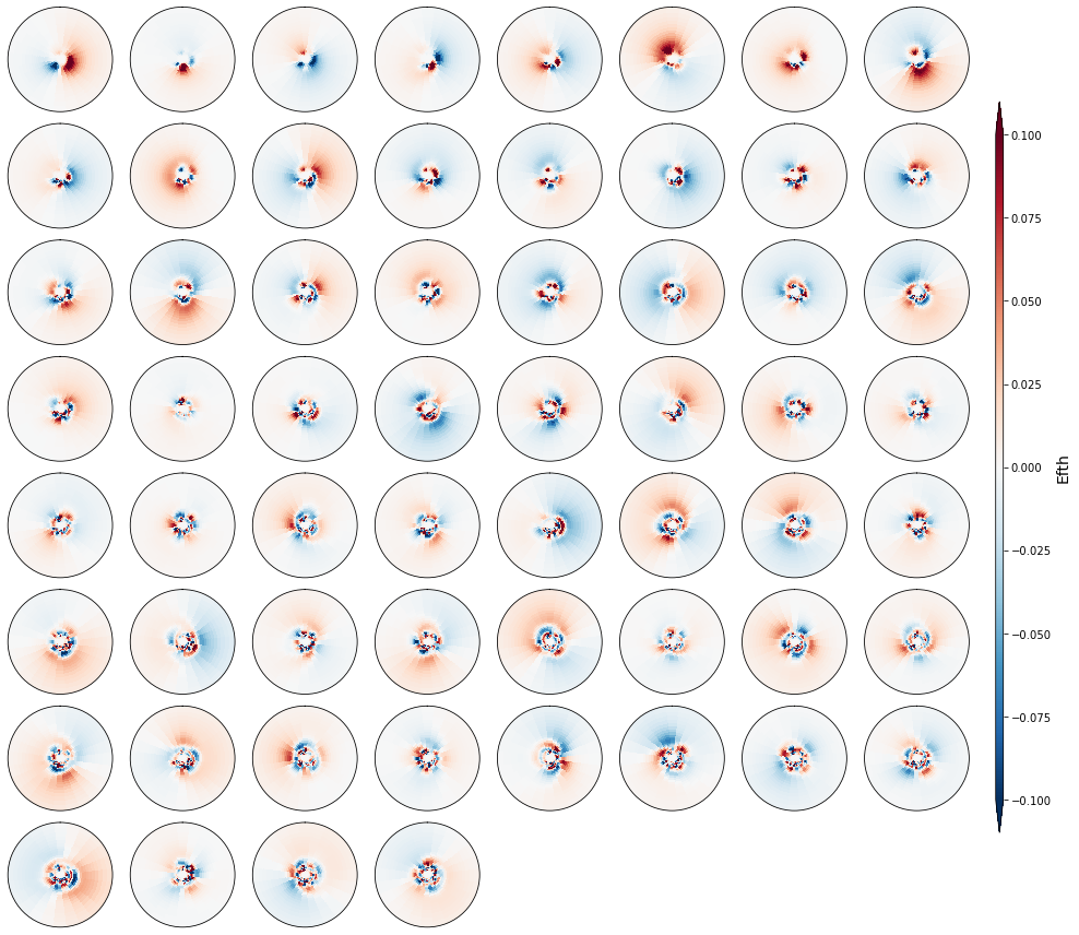
Principal component analysis (PCA), is employed to reduce the high dimensionality of the original data space and simplify the classification process, transforming the information of the full directional spectra into its spatial and temporal modes.
PCA projects the original data on a new space searching for the maximum variance of the sample data.
The PCs represent the temporal variability.
The Empirical Orthogonal Functions, (EOFs) of the data covariance matrix define the vectors of the new space.
The EOFs represent the spatial variability.
In order to classify the spectra following KMA, we keep the n PCs that represent 95% of the explained variance (EV).
# Convert spec data into a matrix (time x (freq * dir))
m = np.reshape(np.sqrt(sp.efth.values), (len(sp.time), len(sp.freq) * len(sp.dir)))
p = 95 # explained variance

ipca = PCA(n_components = np.shape(m)[1])
pk.dump(ipca.fit(m), open(p_spec_pca, 'wb'))

# add PCA data to superpoint
sp['PCs'] =  (('time','pc'), ipca.fit_transform(m))
sp['EOFs'] = (('pc','components'), ipca.components_)
sp['pc'] =   range(np.shape(m)[1])
sp['EV'] =   (('pc'), ipca.explained_variance_)

APEV = np.cumsum(sp.EV.values) / np.sum(sp.EV.values) * 100.0
n_pcs = np.where(APEV > p)[0][0]
sp['n_pcs'] = n_pcs

print('Number of PCs explaining {0}% of the EV is: {1}'.format(p, n_pcs))
Number of PCs explaining 95% of the EV is: 60
# Plot PCs spectra
Plot_spectra_pcs(sp, n_pcs, figsize = [14, 12]);
K-Means Clustering#
K-Means
Spectral clusters are obtained using the K-means clustering algorithm. We divide the data space into 2000 clusters, a number that must be a compromise between the available data to populate the different clusters, and a number large enough for capturing the full variability of the spectra.
Each cluster is defined by a prototype and formed by the data for which the prototype is the nearest. The centroid, which is the mean of all the data that falls within the same cluster, is then represented into a lattice following a geometric criteria, so that similar clusters are placed next to each other for a more intuitive visualization
# minimun data for each cluster
min_data_frac = 100
min_data = np.int(len(sp.time) / num_clusters / min_data_frac)

# KMeans clustering for spectral data
kma, kma_order, bmus, sorted_bmus, centers = kmeans_clustering_pcs(
    sp.PCs.values[:], n_pcs, num_clusters, min_data = min_data,
    kma_tol = 0.001, kma_n_init = 5,
)

# store kma output
pk.dump([kma, kma_order, bmus, sorted_bmus, centers], open(p_spec_kma, 'wb'))


# load kma output
#kma, kma_order, bmus, sorted_bmus, centers = pk.load(open(p_spec_kma, 'rb'))
Iteration: 0
Number of sims: 115
Minimum number of data: 3
# add KMA data to superpoint
sp['kma_order'] =  kma_order
sp['n_pcs'] =  n_pcs
sp['bmus'] = (('time'), sorted_bmus)
sp['centroids'] = (('clusters', 'n_pcs_'), centers)
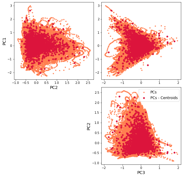
The resulting classification can be seen in the first PCs space, through a scatter plot of PCs and the representative KMA centroids. The obtained centroids (red dots), span the wide variability of the data.
Scatter plot of PCs and the representative KMA centroids:
Plot_pc_space(sp);
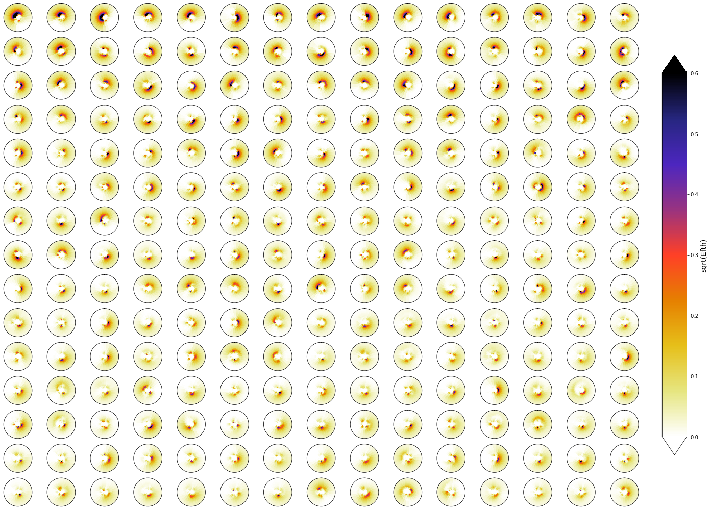
Mean#
The mean spectra associated to each of the different clusters is shown below.
Plot_kmeans_clusters(sp, vmax=0.6, num_clusters=225, ylim=0.3, figsize=[22, 14]);
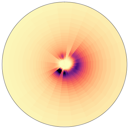
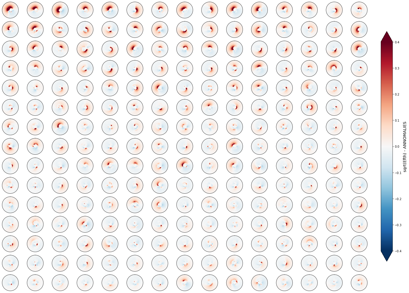
Anomaly#
This is the mean from which annomalies are calculated
z = np.sqrt(np.mean(sp.efth.values, axis=0))
fig = plt.figure(figsize = [8, 8])
ax = fig.add_subplot(1,1,1, projection = 'polar')

y = sp.freq.values
x = np.deg2rad(sp.dir.values)

axplot_spectrum(
    ax,
    x, y, z,
    vmin = 0, vmax = 0.2,
    ylim = np.nanmax(sp.freq),
    remove_axis = 1,
    cmap = 'magma_r',
);
Plot_kmeans_clusters(sp, annomaly=True, vmax=0.4, ylim=0.3, num_clusters=225, figsize=[22, 14]);
# calculate mean from KMeans clusters
efth_clust = calculate_mean_clusters(sp, annomaly=False)

# add mean to superpoint
sp['efth_cluster'] = (('freq', 'dir', 'clusters'), efth_clust)
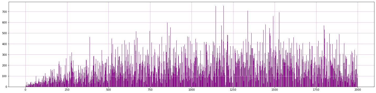
# Plot counts of data inside clusters
values, counts = np.unique(sp.bmus.values, return_counts=True)

plt.figure(figsize = [25, 6])
plt.bar(values, counts, color='darkmagenta')
plt.grid('both', color='plum')
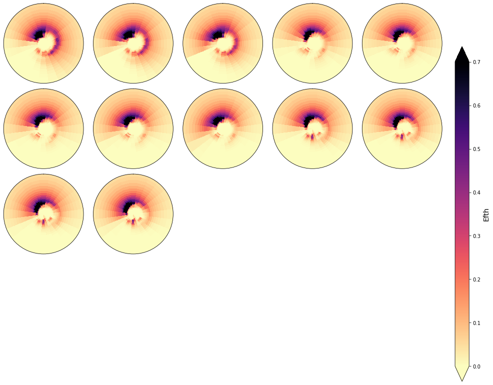
Cluster homogeneity
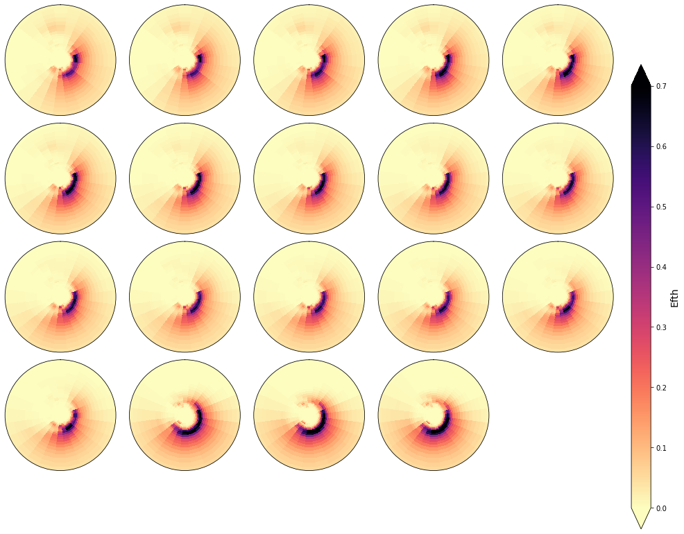
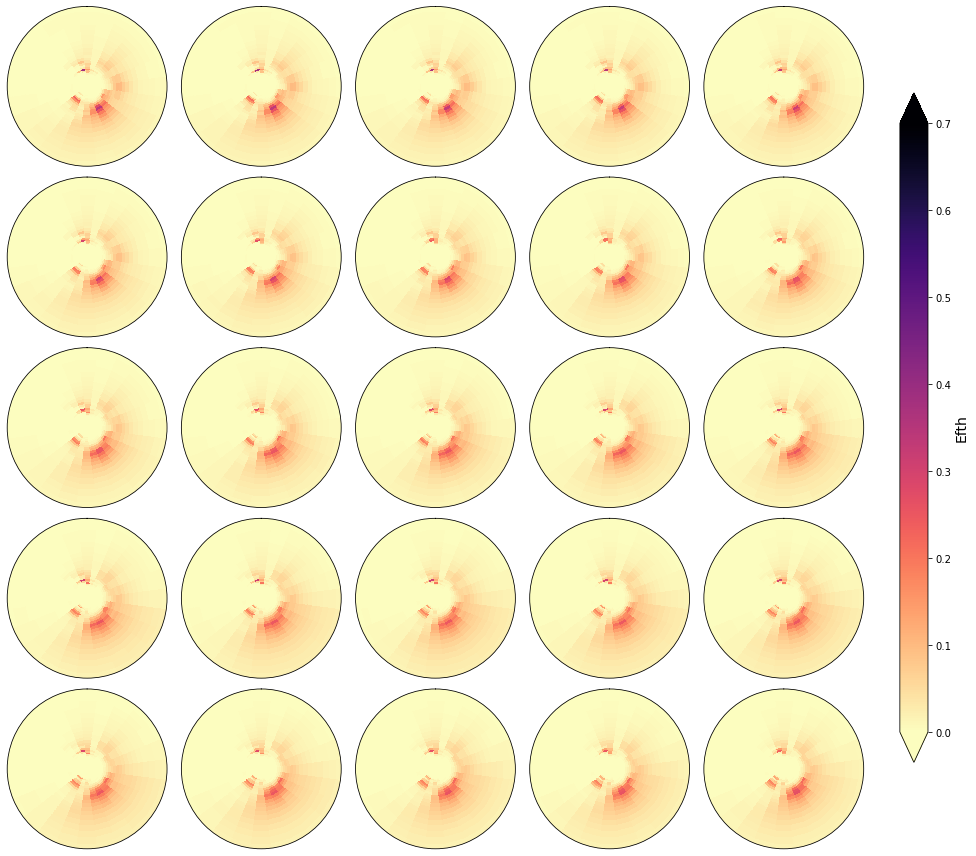
In the following figures, the spectra that fall in the same cluster have been plotted, to validate the homogeneity within each cluster.
As it can be observed, the classification correctly groups the different spectra and the differences within groups are almost negligible
cluster = 1
Plot_specs_inside_cluster(sp, cluster, gr=5, vmax=0.7);
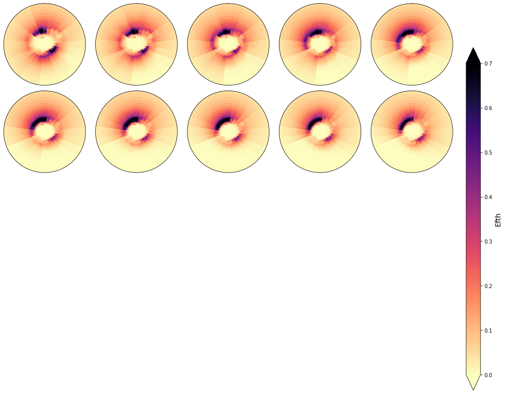
cluster = 16
Plot_specs_inside_cluster(sp, cluster, gr=5, vmax=0.7);
cluster = 40
Plot_specs_inside_cluster(sp, cluster, gr=5, vmax=0.7);
cluster = 600
Plot_specs_inside_cluster(sp, cluster, gr=5, vmax=0.7);
cluster = 1800
Plot_specs_inside_cluster(sp, cluster, gr=5, vmax=0.7);

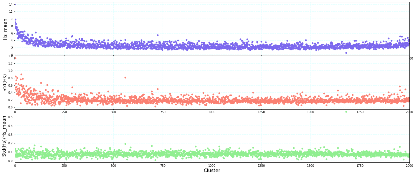
Statistics of Hs within each group#
A quantitative analysis of those differences has been made, analyzing the standard deviation of the Hs representative of each cluster against the mean of the cluster. The results indicate a very low relationship, which means that the clusters are homogeneus.
import wavespectra

sp['Hs'] = sp.efth.spec.hs()
sp
<xarray.Dataset>
Dimensions:       (clusters: 2000, components: 696, dir: 24, freq: 29, kma_order: 2000, n_pcs_: 60, pc: 696, time: 366477)
Coordinates:
  * time          (time) datetime64[ns] 1979-01-01 ... 2020-10-01
  * dir           (dir) float32 262.5 247.5 232.5 217.5 ... 307.5 292.5 277.5
  * freq          (freq) float32 0.035 0.0385 0.04235 ... 0.4171 0.4589 0.5047
  * pc            (pc) int64 0 1 2 3 4 5 6 7 ... 688 689 690 691 692 693 694 695
  * kma_order     (kma_order) int64 318 187 1289 761 1648 ... 222 565 1690 841
Dimensions without coordinates: clusters, components, n_pcs_
Data variables:
    efth          (time, freq, dir) float64 0.0 0.0 0.0 ... 1.464e-05 1.636e-05
    Wspeed        (time) float32 ...
    Wdir          (time) float32 ...
    Depth         (time) float32 ...
    PCs           (time, pc) float64 -0.1756 -0.2968 ... 1.249e-06 2.14e-07
    EOFs          (pc, components) float64 -6.575e-05 -0.0001366 ... -7.586e-05
    EV            (pc) float64 0.1626 0.1375 0.09958 ... 1.052e-10 1.589e-11
    n_pcs         int64 60
    bmus          (time) float64 1.68e+03 1.68e+03 ... 1.803e+03 1.803e+03
    centroids     (clusters, n_pcs_) float64 0.006685 -0.0671 ... 0.03855
    efth_cluster  (freq, dir, clusters) float64 0.0 9.745e-06 ... 1.55e-05
Hs (time) float64 0.0 0.1002 0.17 0.2146 ... 2.524 2.499 2.474- clusters: 2000
- components: 696
- dir: 24
- freq: 29
- kma_order: 2000
- n_pcs_: 60
- pc: 696
- time: 366477
- time(time)datetime64[ns]1979-01-01 ... 2020-10-01
array(['1979-01-01T00:00:00.000000000', '1979-01-01T01:00:00.000000000', '1979-01-01T02:00:00.000000000', ..., '2020-09-30T22:00:00.000000000', '2020-09-30T23:00:00.000000000', '2020-10-01T00:00:00.000000000'], dtype='datetime64[ns]') - dir(dir)float32262.5 247.5 232.5 ... 292.5 277.5
array([262.5, 247.5, 232.5, 217.5, 202.5, 187.5, 172.5, 157.5, 142.5, 127.5, 112.5, 97.5, 82.5, 67.5, 52.5, 37.5, 22.5, 7.5, 352.5, 337.5, 322.5, 307.5, 292.5, 277.5], dtype=float32) - freq(freq)float320.035 0.0385 ... 0.4589 0.5047
array([0.035 , 0.0385 , 0.04235 , 0.046585, 0.051244, 0.056368, 0.062005, 0.068205, 0.075026, 0.082528, 0.090781, 0.099859, 0.109845, 0.12083 , 0.132912, 0.146204, 0.160824, 0.176907, 0.194597, 0.214057, 0.235463, 0.259009, 0.28491 , 0.313401, 0.344741, 0.379215, 0.417136, 0.45885 , 0.504735], dtype=float32) - pc(pc)int640 1 2 3 4 5 ... 691 692 693 694 695
array([ 0, 1, 2, ..., 693, 694, 695])
- kma_order(kma_order)int64318 187 1289 761 ... 565 1690 841
array([ 318, 187, 1289, ..., 565, 1690, 841])
- efth(time, freq, dir)float640.0 0.0 0.0 ... 1.464e-05 1.636e-05
array([[[0.000000e+00, 0.000000e+00, ..., 0.000000e+00, 0.000000e+00], [0.000000e+00, 0.000000e+00, ..., 0.000000e+00, 0.000000e+00], ..., [0.000000e+00, 0.000000e+00, ..., 0.000000e+00, 0.000000e+00], [0.000000e+00, 0.000000e+00, ..., 0.000000e+00, 0.000000e+00]], [[0.000000e+00, 0.000000e+00, ..., 0.000000e+00, 0.000000e+00], [0.000000e+00, 0.000000e+00, ..., 0.000000e+00, 0.000000e+00], ..., [3.714003e-08, 5.114483e-08, ..., 6.950902e-09, 4.801164e-08], [4.271626e-05, 7.017616e-05, ..., 1.037886e-05, 2.627496e-05]], ..., [[0.000000e+00, 0.000000e+00, ..., 0.000000e+00, 0.000000e+00], [4.784205e-08, 5.337963e-08, ..., 7.736124e-13, 6.761713e-09], ..., [4.012885e-05, 5.771459e-05, ..., 3.528962e-05, 3.433209e-05], [2.478915e-05, 3.696030e-05, ..., 2.073825e-05, 2.077800e-05]], [[0.000000e+00, 0.000000e+00, ..., 0.000000e+00, 0.000000e+00], [4.918568e-08, 5.067912e-08, ..., 1.211514e-12, 7.301099e-09], ..., [3.615466e-05, 5.864479e-05, ..., 2.559555e-05, 2.719132e-05], [2.312578e-05, 3.814447e-05, ..., 1.464055e-05, 1.636022e-05]]]) - Wspeed(time)float32...
[366477 values with dtype=float32]
- Wdir(time)float32...
[366477 values with dtype=float32]
- Depth(time)float32...
[366477 values with dtype=float32]
- PCs(time, pc)float64-0.1756 -0.2968 ... 2.14e-07
array([[-1.75569171e-01, -2.96828335e-01, 8.28249588e-01, ..., -8.36433281e-07, 2.76050213e-07, -1.20604521e-07], [-1.75656783e-01, -2.96809334e-01, 8.28244335e-01, ..., -1.72018209e-06, 2.87707831e-07, -5.82479394e-08], [-1.75766723e-01, -2.96745790e-01, 8.28178430e-01, ..., -1.58022234e-06, -3.19978653e-07, 2.76542212e-08], ..., [-5.12250210e-01, -2.09257083e-01, -1.95153881e-01, ..., -2.16666580e-06, 2.71633225e-06, 4.78258709e-07], [-5.17464127e-01, -1.99269416e-01, -2.09358481e-01, ..., -1.09770146e-06, 2.27907312e-06, 3.14019089e-07], [-5.24368669e-01, -1.89185397e-01, -2.22569343e-01, ..., -4.84349416e-07, 1.24879492e-06, 2.14021651e-07]]) - EOFs(pc, components)float64-6.575e-05 ... -7.586e-05
array([[-6.57498085e-05, -1.36630393e-04, -4.20240451e-04, ..., -1.16072261e-03, -1.46509351e-03, -1.88567619e-03], [-1.64548627e-05, -5.64908832e-05, 8.42307218e-05, ..., -7.21854278e-04, -4.71277252e-04, -2.79624691e-04], [-1.67010011e-04, -3.58245086e-04, -8.15555109e-04, ..., 1.82177325e-03, 1.45229700e-03, 9.98281489e-04], ..., [-2.65288192e-03, 9.63100820e-05, -1.73041197e-05, ..., 2.07879006e-04, 1.38560081e-04, -2.96060168e-04], [ 4.74294642e-04, 1.76834888e-04, 6.45303859e-05, ..., -8.37919859e-04, 7.46380579e-04, 1.37141168e-04], [ 2.29787222e-04, -5.43320155e-05, 1.83876037e-05, ..., -1.82500332e-05, -8.93812969e-06, -7.58589172e-05]]) - EV(pc)float640.1626 0.1375 ... 1.589e-11
array([1.62631313e-01, 1.37462889e-01, 9.95776054e-02, 8.21767604e-02, 5.26271564e-02, 4.11897801e-02, 3.93639040e-02, 3.76972294e-02, 3.15263798e-02, 2.27256479e-02, 2.07069062e-02, 1.93208019e-02, 1.70484693e-02, 1.47094104e-02, 1.24071042e-02, 1.15477288e-02, 1.05804252e-02, 1.01850639e-02, 9.09891223e-03, 8.56244103e-03, 8.28225396e-03, 7.31750264e-03, 6.72686195e-03, 6.58608391e-03, 6.29213260e-03, 6.09061851e-03, 5.46009858e-03, 5.20802867e-03, 4.88901930e-03, 4.63520711e-03, 4.46851326e-03, 4.29470592e-03, 3.95994782e-03, 3.74811195e-03, 3.64100535e-03, 3.52618679e-03, 3.45065451e-03, 3.30612798e-03, 2.98593680e-03, 2.77445413e-03, 2.69739472e-03, 2.64890592e-03, 2.55704794e-03, 2.51031489e-03, 2.34345690e-03, 2.25139662e-03, 2.20354588e-03, 2.16838876e-03, 2.06107523e-03, 1.98629381e-03, 1.82304081e-03, 1.79259689e-03, 1.72350073e-03, 1.65675046e-03, 1.54064512e-03, 1.51876384e-03, 1.48209230e-03, 1.45041228e-03, 1.39592227e-03, 1.34972009e-03, 1.32136008e-03, 1.28189268e-03, 1.21614820e-03, 1.14665817e-03, 1.08515718e-03, 1.07557680e-03, 1.05635305e-03, 1.01427749e-03, 9.85901093e-04, 9.72768436e-04, 9.59804795e-04, 9.51656998e-04, 9.31656904e-04, 8.50521763e-04, 8.26692154e-04, 7.79465830e-04, 7.68369130e-04, 7.59021532e-04, 7.42014827e-04, 7.23539074e-04, ... 1.85727999e-08, 1.81928930e-08, 1.70481732e-08, 1.69700618e-08, 1.67501829e-08, 1.54614890e-08, 1.51824540e-08, 1.50149697e-08, 1.46406234e-08, 1.43272291e-08, 1.42065050e-08, 1.38627491e-08, 1.33565658e-08, 1.31388966e-08, 1.27471913e-08, 1.25137819e-08, 1.22831649e-08, 1.18871094e-08, 1.17980644e-08, 1.14186368e-08, 1.10501821e-08, 1.09971176e-08, 1.07990339e-08, 1.06415617e-08, 1.04931942e-08, 1.02496609e-08, 9.84863177e-09, 9.69794482e-09, 8.93555986e-09, 8.63235425e-09, 8.43968651e-09, 8.11093289e-09, 7.34358544e-09, 7.18776398e-09, 7.03955683e-09, 6.71324185e-09, 6.39290570e-09, 6.21916537e-09, 6.11239150e-09, 5.68430954e-09, 5.48051520e-09, 5.27405993e-09, 5.21129195e-09, 5.11015912e-09, 4.80550444e-09, 4.77360454e-09, 4.16135224e-09, 3.98013321e-09, 3.85355716e-09, 3.71949655e-09, 3.64122228e-09, 3.54038656e-09, 3.24461532e-09, 3.21424037e-09, 3.13683100e-09, 3.07680989e-09, 2.96197885e-09, 2.90132644e-09, 2.78700916e-09, 2.60032368e-09, 2.41637919e-09, 2.25833729e-09, 2.12286128e-09, 1.98978753e-09, 1.84178693e-09, 1.78690786e-09, 1.54677487e-09, 1.38987663e-09, 1.37098113e-09, 1.31828472e-09, 1.17110222e-09, 1.11847527e-09, 1.04045076e-09, 9.10463255e-10, 8.51224318e-10, 3.18195175e-10, 2.89491697e-10, 2.07637291e-10, 1.05249600e-10, 1.58939092e-11]) - n_pcs()int6460
array(60)
- bmus(time)float641.68e+03 1.68e+03 ... 1.803e+03
array([1680., 1680., 1680., ..., 1803., 1803., 1803.])
- centroids(clusters, n_pcs_)float640.006685 -0.0671 ... 0.03855
array([[ 6.68452222e-03, -6.70987084e-02, 3.20171828e-01, ..., 5.01826122e-02, 1.95730391e-03, -1.45509414e-02], [-5.20134784e-01, -6.70128930e-02, -2.27595628e-01, ..., -1.34278897e-02, -7.41491375e-04, 5.61174938e-03], [-6.49631429e-01, 1.09320965e+00, -2.60207927e-01, ..., 2.01649530e-02, -3.66295422e-03, -1.06885357e-02], ..., [ 3.02901297e-01, 4.02556666e-01, 9.11489904e-02, ..., -1.38198024e-02, -2.77484137e-02, -4.20207027e-03], [ 8.27634243e-01, 1.45795289e-01, -2.33225251e-01, ..., 5.33047247e-03, 4.96915811e-02, -7.29735073e-03], [-2.49641668e-01, -1.70728296e-01, 2.31709086e-01, ..., -1.22055822e-01, 2.23503320e-02, 3.85490949e-02]]) - efth_cluster(freq, dir, clusters)float640.0 9.745e-06 ... 1.55e-05
array([[[0.00000000e+00, 9.74493783e-06, 0.00000000e+00, ..., 4.35874773e-08, 4.47661048e-08, 1.00230523e-07], [0.00000000e+00, 1.38885975e-06, 0.00000000e+00, ..., 4.53452682e-08, 2.80266308e-07, 5.85710898e-08], [0.00000000e+00, 1.99842969e-08, 0.00000000e+00, ..., 3.41219840e-06, 9.70217354e-07, 9.33574001e-07], ..., [0.00000000e+00, 8.01385027e-09, 0.00000000e+00, ..., 3.36690930e-09, 6.76305482e-09, 1.63439162e-09], [0.00000000e+00, 3.04449492e-07, 0.00000000e+00, ..., 1.94692591e-09, 1.31829637e-10, 3.75291419e-10], [0.00000000e+00, 2.00873861e-05, 0.00000000e+00, ..., 2.46300616e-08, 1.50312293e-08, 1.93432277e-08]], [[9.87308252e-04, 1.59755295e-04, 2.78248499e-07, ..., 5.41070956e-06, 1.53992578e-06, 5.49980010e-06], [6.41497016e-05, 1.53704480e-05, 3.92092156e-08, ..., 5.38487605e-06, 1.12629101e-05, 6.02034319e-06], [6.42977640e-06, 6.59273419e-07, 2.00163807e-05, ..., 4.26830712e-05, 5.14788839e-05, 2.17147743e-05], ... [8.06043593e-04, 4.12587341e-04, 4.65747723e-04, ..., 5.99360541e-05, 2.17599883e-06, 3.35727696e-05], [7.62885348e-04, 3.23912588e-04, 5.12386223e-04, ..., 7.18552580e-05, 2.99060853e-06, 2.80055703e-05], [5.51892420e-04, 1.69104720e-04, 5.66123018e-04, ..., 9.40061488e-05, 4.56541857e-06, 2.44764382e-05]], [[2.98285612e-04, 5.58369091e-05, 3.69578159e-04, ..., 7.58942491e-05, 4.00281898e-06, 1.26926651e-05], [2.37153442e-04, 7.89735714e-06, 3.89739614e-04, ..., 9.48134722e-05, 5.58493447e-06, 1.22437544e-05], [2.09787389e-04, 9.41177875e-07, 3.49983569e-04, ..., 1.00451678e-04, 8.46082909e-06, 1.19207556e-05], ..., [5.24764458e-04, 2.68257351e-04, 2.99670603e-04, ..., 3.61587916e-05, 1.39305010e-06, 2.19963861e-05], [4.98467180e-04, 2.08217319e-04, 3.30764575e-04, ..., 4.51528194e-05, 1.94257293e-06, 1.77920584e-05], [3.59868019e-04, 1.05412218e-04, 3.68032305e-04, ..., 6.12963415e-05, 3.03584193e-06, 1.54973520e-05]]]) - Hs(time)float640.0 0.1002 0.17 ... 2.499 2.474
- standard_name :
- sea_surface_wave_significant_height
- units :
- m
array([0.        , 0.10015632, 0.17001594, ..., 2.52396895, 2.49886996,
       2.4735167 ])
Plot_kmeans_hs_stats(sp, figsize=[24, 10]);
# store modified superpoint with KMA data
sp.to_netcdf(p_superpoint_kma)