Super Point Definition

In order to account for all the possible energy and to avoid the shadowing effect due to land presence, the first step consists on defining a super-point (Cagigal et al., 2021), which aggregated the energy from a number of points surrounding the study site.

This virtual super-point has been constructed using the directional spectra from the CAWCR (Centre for Australian Weather and Climate Research) hindcast (Durrant et al., 2014; Smith et al., 2020), which provides spectral data at 10° resolution for the global grid, and 0.5° for the Pacific Region, in which our study is located.

# common
import warnings
warnings.filterwarnings('ignore')
import os
import os.path as op
import sys

# pip
import xarray as xr
import numpy as np

# DEV: bluemath
sys.path.insert(0, op.join(op.abspath(''), '..', '..', '..', '..'))

# bluemath modules
from bluemath.superpoint.spectra import stations_superposition, bulkparams_partitions
from bluemath.superpoint.plotting.stations import Plot_stations
from bluemath.superpoint.plotting.spectra import Plot_stations_spectra, Plot_spectrum, Plot_seasons_spectra
from bluemath.superpoint.plotting.bulk_parameters import Plot_bulk_parameters, Plot_partitions

from bluemath.plotting.nearshore import Plot_obstructions_CAWCR

Database and site parameters

# database
p_data = r'/media/administrador/HD2/SamoaTonga/data'
p_resources = r'/media/administrador/HD2/SamoaTonga/resources'
site='Tongatapu'
p_site = op.join(p_data, site)

# input stations
p_stat = op.join(p_site, 'stations')

# deliverable folder
p_deliv = op.join(p_site, 'd05_swell_inundation_forecast')

p_spec = op.join(p_deliv, 'spec')
p_figs = op.join(p_deliv, 'figs')

# CAWCR obstructions
p_obstr_cawcr = op.join(p_resources, 'ww3_grid_inputs', 'Obstructions_CAWCR.nc')


# SUPERPOINT parameters
deg_sup         = 15  # degrees of superposition
stations_id=[1938,1939,1921,1920,1919,1937]
stations_sector=[(330,30),(30,90),(90,150),(150,210),(210,270),(270,330)]

stations_pos=[5,0,1,4,3,2] #positions of the stations for plotting
st_wind=1939
lat_p=-21.22
lon_p=-175.07

# WAVESPECTRA parameters
part0 = True           # False if we dont want a sea partition (that will change wind to 0)
wcut  = 0.00000000001  # wind cut
msw   = 8              # max number of swells
agef  = 1.7            # age Factor
model = 'csiro'


# output files
p_superpoint = op.join(p_spec, 'super_point_superposition_{0}_.nc'.format(deg_sup))
p_chunks = op.join(p_spec, 'chunks')
p_partitions = op.join(p_spec, 'partitions_stats_wcut_{0}_.nc'.format(wcut))
p_bulk = op.join(p_spec, 'bulk_params_wcut_{0}_.nc'.format(wcut))


# make data folders
for f in [p_deliv, p_spec, p_figs]:
    if not op.isdir(f):
        os.makedirs(f)

Motivation

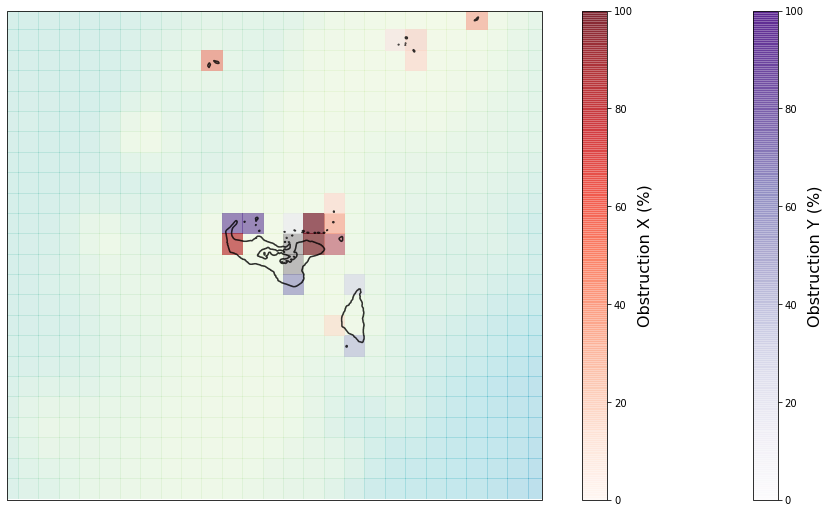
CAWCR obstructions

Below, a plot of the obstructions included in the CAWCR global wave hindcast is included.

• Grey cells correspond to land
  

• Red and purple cells correspond to obstructions in the X and Y direction respectively.
  
  The misinterpretation of island settings puts into evidence the need of performing a detailed downscaling of the wave dynamics.
  

# load CAWCR obstructions
obstr_cawcr = xr.open_dataset(p_obstr_cawcr)

# plot CAWCR obstructions
Plot_obstructions_CAWCR(
    obstr_cawcr, 
    area = [lon_p -1 + 360, lon_p + 0.75 + 360, lat_p - 0.75, lat_p + 0.85], 
    figsize = [18, 9],
);

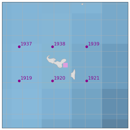
Constructing the “Super Point”

Location of the selected stations used for the Super Point construction. Each station will represent one directional sector of the Super-Point spectra

# plot Super Point stations
fig = Plot_stations(
    p_stat, stations_id, 
    lon_p = lon_p, lat_p = lat_p,
    extra_area = 1, 
    figsize = [12, 8],
)

# store figure
p_f = op.join(p_figs, 'stations_'+site+'.png')
fig.savefig(p_f, dpi = 600, transparent = True)

# Super Point stations superposition
super_point = stations_superposition(p_stat, stations_id, stations_sector, deg_sup, st_wind)
super_point.to_netcdf(p_superpoint)  

#super_point = xr.open_dataset(p_superpoint)

# remove wind so no sea partition is created
if not part0:
    super_point.Wspeed.values = np.zeros(np.shape(super_point.Wspeed.values))

print(super_point)

Station: 1938
Station: 1939
Station: 1921
Station: 1920
Station: 1919
Station: 1937
<xarray.Dataset>
Dimensions:  (dir: 24, freq: 29, time: 366477)
Coordinates:
  * time     (time) datetime64[ns] 1979-01-01 1979-01-01T01:00:00 ... 2020-10-01
  * dir      (dir) float32 262.5 247.5 232.5 217.5 ... 322.5 307.5 292.5 277.5
  * freq     (freq) float32 0.035 0.0385 0.04235 ... 0.4171 0.4589 0.5047
Data variables:
    efth     (time, freq, dir) float64 0.0 0.0 0.0 ... 1.464e-05 1.636e-05
    Wspeed   (time) float32 3.892 3.892 3.922 3.961 ... 3.783 3.809 4.351 5.321
    Wdir     (time) float32 285.8 285.8 279.1 271.1 ... 250.8 231.7 209.8 193.5
    Depth    (time) float32 1.167e+03 1.167e+03 ... 1.167e+03 1.167e+03

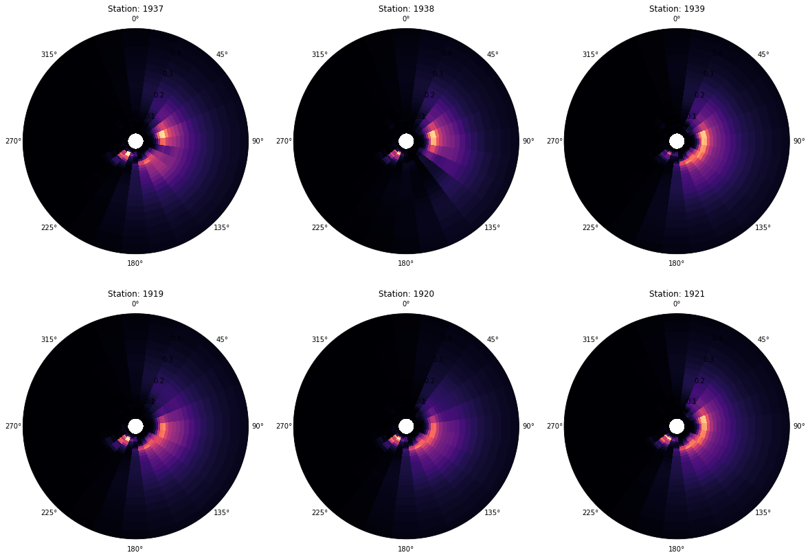
Here is an example for a specific time:

time_index = 5000

This is the spectr at each of the different stations at the same time:

The shadowing effect of the island is clear for some directions, which emphasized the importance of constructing the Super Point in order to capture all the energy arrivign towards our study site.

Plot_stations_spectra(
    p_stat, stations_id, stations_pos,
    time_index,
    gs_rows = 2, gs_cols = 3,
    figsize = [20, 14],
);

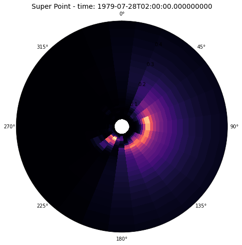
This is the Super-Point at that time:

Plot_spectrum(super_point, time_index);

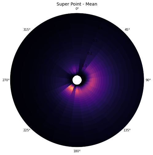
Mean Super-Point spectrum for the period 1979-2020:

Plot_spectrum(super_point, average=True);

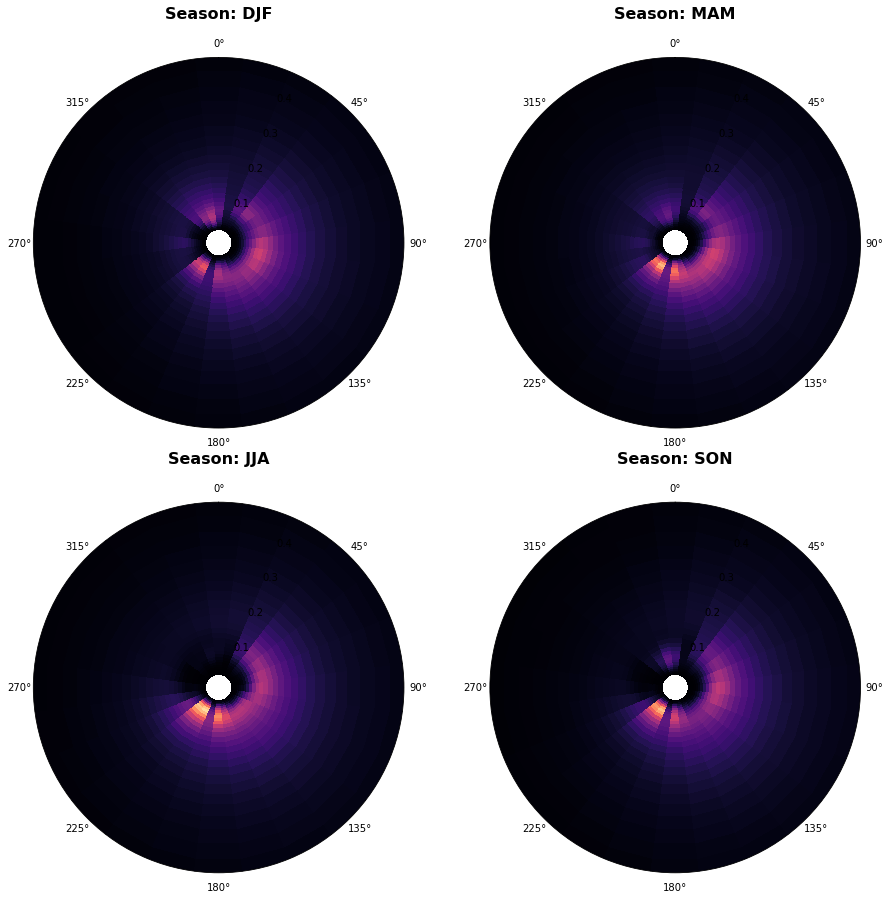
Mean spectrum by season:

Plot_seasons_spectra(super_point);

Obtention of bulk parameters and partitions*

Once the Super-Point is defined, we obtain the representative partitions and bulk parameters by means of the library wavespectra (https://github.com/metocean/wavespectra)

Nevertheless, bulk parameters and/or partitions will not be used for constructing the seasonal forecast

# obtain superpoint partitons and bulk parameters
bulk_params, stats_part = bulkparams_partitions(
    p_chunks, super_point, chunks=3, 
    wcut=wcut, msw=msw, agef=agef,
)

# store partitions and bulk parameters
bulk_params.to_netcdf(p_bulk)
stats_part.to_netcdf(p_partitions)

#bulk_params = xr.open_dataset(p_bulk)
#stats_part = xr.open_dataset(p_partitions)

Warning: cannot import cf-json, install "metocean" dependencies for full functionality
chunk 1/3 done.
chunk 2/3 done.
chunk 3/3 done.

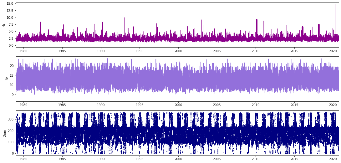
Bulk parameters:

Plot_bulk_parameters(bulk_params);

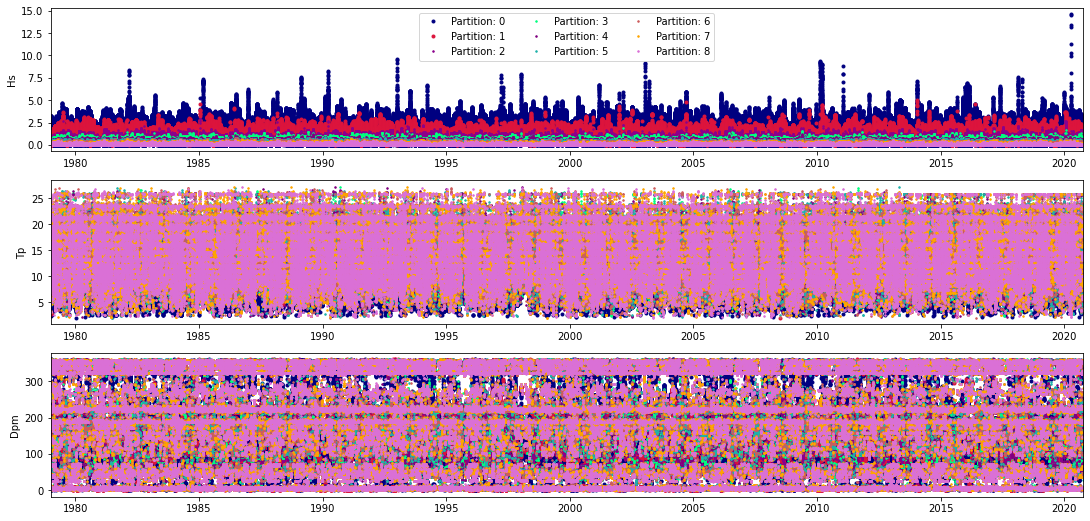
Partitions:

Plot_partitions(stats_part, num_fig=1);