KMA Reconstruction
Contents
KMA Reconstruction#
# common
import warnings
warnings.filterwarnings('ignore')
import os
import os.path as op
import sys
import pickle as pkl

# pip
import xarray as xr
import numpy as np
import pandas as pd
import matplotlib.pyplot as plt

# DEV: bluemath
sys.path.insert(0, op.join(op.abspath(''), '..', '..', '..', '..'))

# bluemath modules
from bluemath.binwaves.reconstruction import generate_kp_coefficients, reconstruct_kmeans_clusters_hindcast, \
                                             load_point_kp, load_point_efth_kma, load_hindcast_recon

from bluemath.binwaves.plotting.swan_case import Plot_swan_case
from bluemath.binwaves.plotting.buoy import Plot_comparison_buoy, Plot_buoy_location
from bluemath.binwaves.plotting.spectra import Plot_example_spectra, Plot_spectra_propagation
Warning: cannot import cf-json, install "metocean" dependencies for full functionality
Database and site parameters#
# database
p_data = '/media/administrador/HD2/SamoaTonga/data'
site = 'Tongatapu'
p_site = op.join(p_data, site)

# deliverable folder
p_deliv = op.join(p_site, 'd05_swell_inundation_forecast')

p_kma = op.join(p_deliv, 'kma')
p_swan = op.join(p_deliv, 'swan')

# SWAN simulation parameters
name = 'binwaves'
p_swan_subset = op.join(p_swan, name, 'subset.nc')
p_swan_output = op.join(p_swan, name, 'out_main_binwaves.nc')
p_swan_input_spec = op.join(p_swan, name, 'input_spec.nc')

# SuperPoint KMeans
num_clusters = 2000
p_superpoint_kma = op.join(p_kma, 'Spec_KMA_{0}_NS.nc'.format(num_clusters))

# buoy data
point_buoy1 = [184.785, -21.221]
p_buoy1=op.join(p_site, 'buoy', 'tongatapu_lon' + str(point_buoy1[0]) + '_' + 'lat' + str(point_buoy1[1]) + '.pkl')

point_buoy2 = [184.730, -21.2370]
p_buoy2 = op.join(p_site, 'buoy','Buoy_' + str(point_buoy2[0]) + '_' + str(point_buoy2[1]) + '.nc')

# output files
p_site_out = op.join(p_deliv, 'reconstruction')

p_kp_coeffs = op.join(p_site_out, 'kp_grid')          # SWAN propagation coefficients
p_efth_kma = op.join(p_site_out, 'efth_kma')          # KMA reconstruction
p_reco_hnd = op.join(p_site_out, 'hindcast')          # hindcast reconstruction folder
SWAN simulations and area#
SWAN Simulation parameters
# Load SWAN simulation parameters
subset = xr.open_dataset(p_swan_subset)
out_sim_swan = xr.open_dataset(p_swan_output).load()
input_spec = xr.open_dataset(p_swan_input_spec)
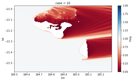
Here we need to define the area for the extraction and the resample factor
The plot is an example of the area that has been cut
# this will reduce memory usage
area_extraction=[184.5, 185.3, -21.62, -20.97]
resample_factor = 2 #1 means no resample

# cut area
out_sim = out_sim_swan.sel(
    lon = slice(area_extraction[0], area_extraction[1]),
    lat = slice(area_extraction[2], area_extraction[3]),
)

# resample extraction points
out_sim = out_sim.isel(
    lon = np.arange(0, len(out_sim.lon), resample_factor),
    lat = np.arange(0, len(out_sim.lat), resample_factor),
)

# check that the area is OK
plt.figure(figsize = [9, 5])
out_sim.isel(case = 10).Hsig.plot(cmap='RdBu', vmin=0, vmax=2);
KMA clusters#
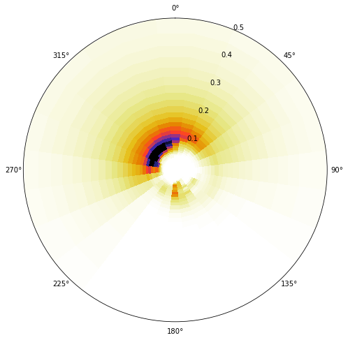
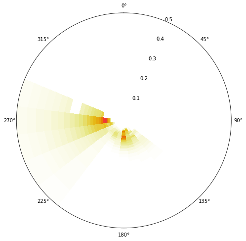
We reconstruct the spec in the grid points, for the 2000 spectral centroids of the cluster
sp_kma = xr.open_dataset(p_superpoint_kma)
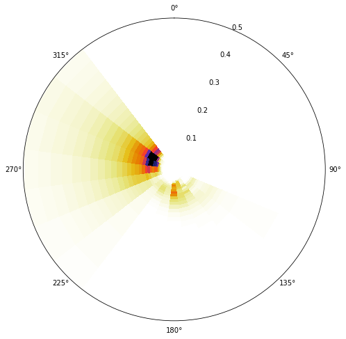
One cluster example OFFSHORE
# example cluster
cluster = 4

# Plot spectra
Plot_example_spectra(sp_kma, cluster=cluster);
Simulations preprocess#
This is where we postprocess all the simulations, to obtain the propagation coefficients (kp) for all the 696 cases and for each point of the grid
This process takes a long time but it only needs to be run once
# generate propagation coefficients for all points and cases
generate_kp_coefficients(p_kp_coeffs, out_sim, sp_kma, override=False)
Preprocessing kp coefficients...: 100%|██████████████████████████████| 30141/301
Explanation
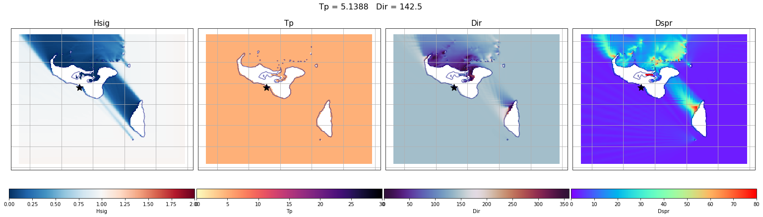
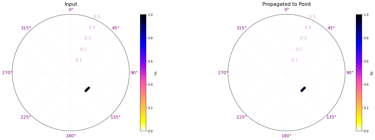
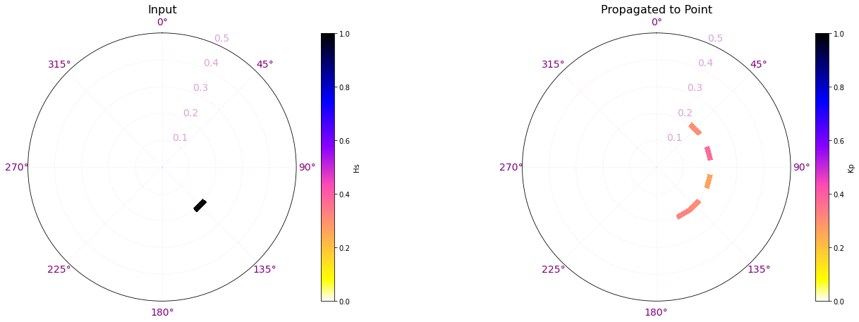
Here are a couple examples of the process made here for one of the propagation cases.
In the plots below, the propagation for a case out of the 696 has been plotted with the propagations for two different points of the grid (The ones marked with a star)
The first example is for the buoy location, which receives all the energy from the 142.5º direction. The Kp coefficient is 1 with the same direction as the input offshore spectra, meaning that any energy is lost.
The second example is for a location in the northern part of Tognatapu, where waves are shadowed by the many small islands in the area. For this reason the same input spectra is here transformed into 4 different systems with different directions, kist a kp coefficient of around 0.1/0.2
# Select one propagation case
case = 250
point_example = [184.785, -21.221]

# Load spectra kp
output_spec = load_point_kp(point_example, out_sim, p_kp_coeffs)

# Plot SWAN case
Plot_swan_case(out_sim, subset, case, point_example[0], point_example[1]);

# Plot SWAN Hs propagation spectra
Plot_spectra_propagation(input_spec, output_spec, sp_kma, case, ylim=0.5, cmap='gnuplot2_r');
# Select one propagation case
case = 250
point_example = [184.91, -21.05]

# Load spectra kp
output_spec = load_point_kp(point_example, out_sim, p_kp_coeffs)

# Plot SWAN case
Plot_swan_case(out_sim, subset, case, point_example[0], point_example[1]);

# Plot SWAN Hs propagation spectra
Plot_spectra_propagation(input_spec, output_spec, sp_kma, case, ylim=0.5, cmap='gnuplot2_r');

Reconstruction based on KMA#
Validation#
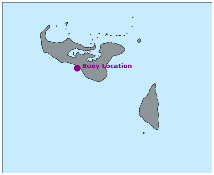
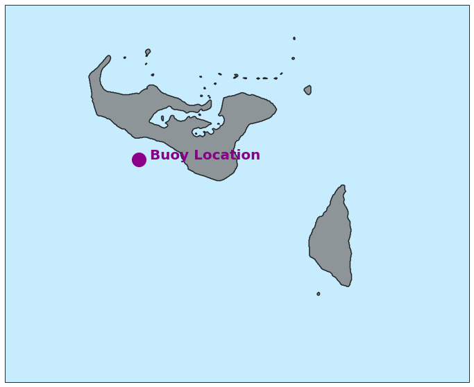
Below is the Buoy Location available for validation at our study site
Buoy Location 1#
# Plot buoy location
Plot_buoy_location(point_buoy1, area_extraction);
# reconstruct model data for that specific point
reconstruct_kmeans_clusters_hindcast(
    p_site_out, out_sim, sp_kma,
    point = point_buoy1,
    reconst_hindcast = True,
    override = False,
)
Preprocessing efth and stats...: 100%|██████████████████████████████| 1/1 [00:00
Same cluster as in the example above, propagated to buoy at Location 1
# Load propagated spectra
efth_point = load_point_efth_kma(point_buoy1, out_sim, p_efth_kma)

# Plot spectra
Plot_example_spectra(efth_point, cluster=cluster);
# load buoy data and parse it to xarray.Dataset
with open(p_buoy1, 'rb') as fr:
    buoy = pkl.load(fr)

buoy_data1 = buoy.to_xarray().isel(index = np.where((buoy.hs > 0) & (buoy.tm10 > 0))[0])
# Load hindcast reconstruction at nearest point to buoy
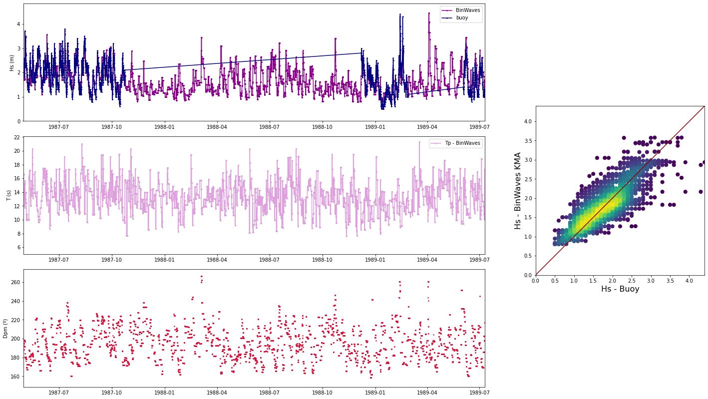
recon_data = load_hindcast_recon(point_buoy1, out_sim, p_reco_hnd)
# compare hindcast reconstruction with buoy data
Plot_comparison_buoy(recon_data, buoy_data1, ss=3);
Buoy Location 2#
# Plot buoy location
Plot_buoy_location(point_buoy2, area_extraction);
# reconstruct model data for that specific point
reconstruct_kmeans_clusters_hindcast(
    p_site_out, out_sim, sp_kma,
    point = point_buoy2,
    reconst_hindcast = True,
    override = False,
)
Preprocessing efth and stats...: 100%|██████████████████████████████| 1/1 [00:00
Same cluster as in the example above, propagated to buoy at Location 1
# Load propagated spectra
efth_point = load_point_efth_kma(point_buoy2, out_sim, p_efth_kma)

# Plot spectra
Plot_example_spectra(efth_point, cluster=cluster);
# load buoy data and parse it to xarray.Dataset

buoy = xr.open_dataset(p_buoy2)
buoy_data2 = buoy.isel(index = np.where((buoy.hs > 0) & (buoy.tm10 > 0))[0])
# Load hindcast reconstruction at nearest point to buoy
recon_data = load_hindcast_recon(point_buoy2, out_sim, p_reco_hnd)
# compare hindcast reconstruction with buoy data
Plot_comparison_buoy(recon_data, buoy_data2, ss=3);
