BinWaves & SWAN#

import warnings
warnings.filterwarnings('ignore')

# common
import os
import os.path as op
import sys
import pickle as pk
import shutil

# pip
import numpy as np
import pandas as pd
import xarray as xr

# DEV: bluemath
sys.path.insert(0, op.join(op.abspath(''), '..', '..', '..', '..'))

# bluemath modules 
from bluemath.common import store_xarray_max_compression

from bluemath.binwaves.plotting.grid import Plot_grid_cells, Plot_grid_cases
from bluemath.binwaves.plotting.swan_case import Plot_swan_case

from bluemath.wswan.wrap import SwanProject, SwanMesh, SwanWrap_STAT
from bluemath.wswan.plots.stationary import scatter_maps

Methodology#

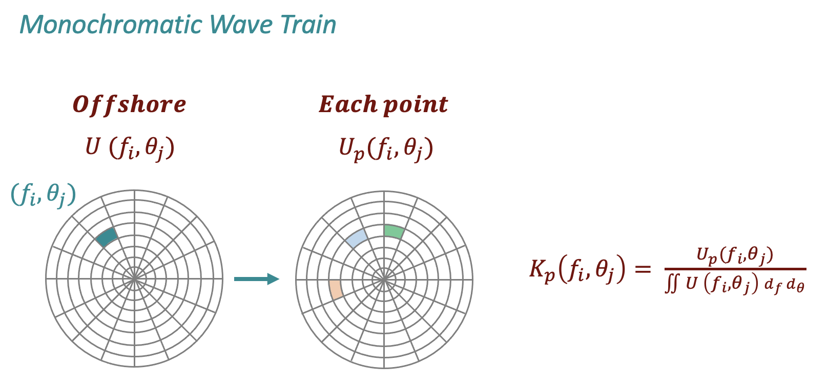
BinWaves

A new methodology for efficiently propagating multivariate wave systems to nearshore locations is propossed.
The methodology, which is named BinWaves, consists on disagregating the full wave spectra into its different energy “bins” which are characterized by monochromatic wave trains represented by a frequency and a direction.
Based on the linearity of the waves in deep waters, every directional spectra can be later on aggregated by supperposing all its different constituents at each location and time.

Methodology

These are the steps followed in the BinWaves methodology

Divide the full energy spectra into its individual energy “bins”. The spectra, characterized by 29 frequencies and 24 directions, results in 696 monochromatic wave trains.
Numerically run the 696 monochromatic cases with unitary significant wave height.
Post process the 696 simulations to obtain the propagation coefficients (Kp) of each energy bin at every location.

The propagation coefficients nearshore, as exemplified in the sketch below at each point of the grid, can be characterized by more than 1 different directional component due to the interaction with the bathymetry along the propagation.

SWAN

Individual “bins” have been numerically simulated using SWAN (Simulating WAves Nearshore), which is a third-generation open source wave model developed at Delft University of Technology.

TITLE

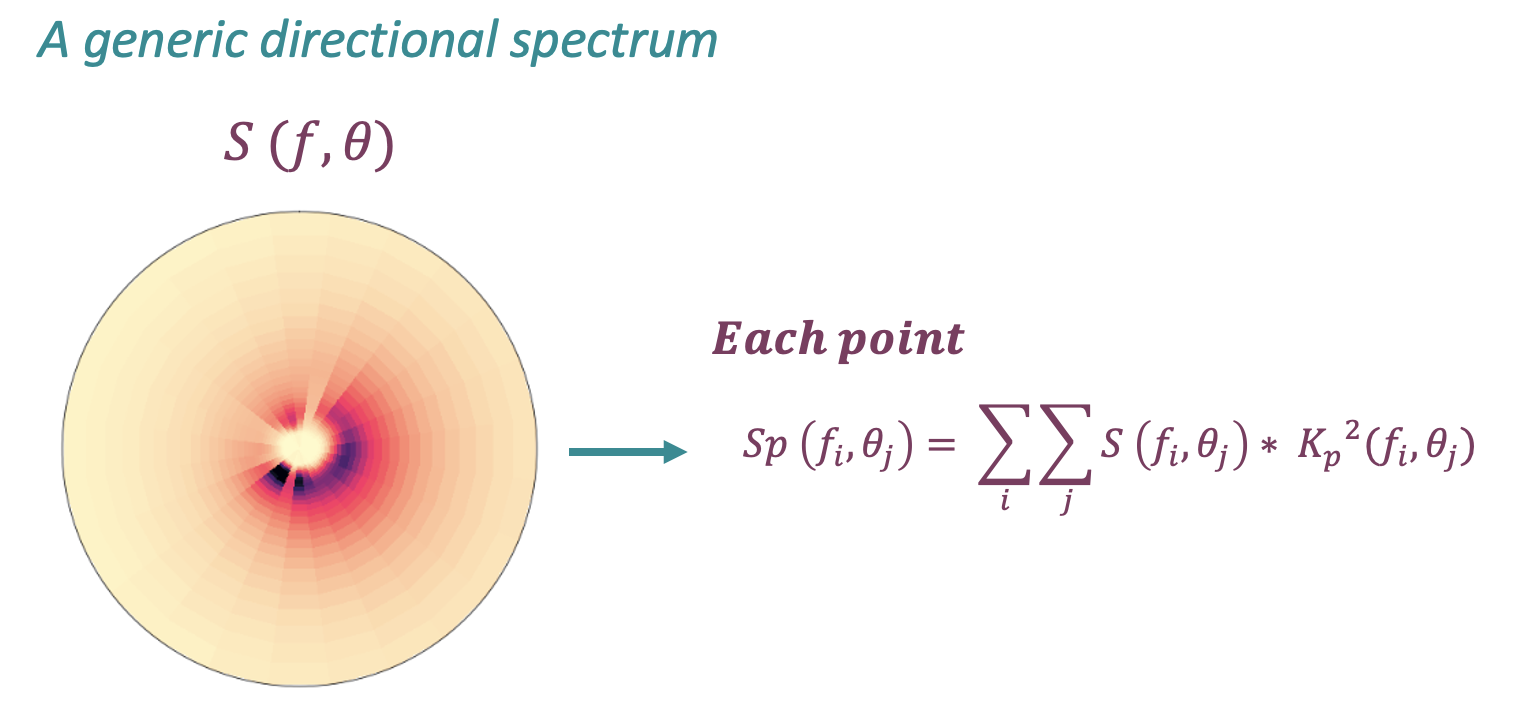
Reconstruction methodology

Once the outputs of the BinWaves methodology have been obtained at each point of the grid, for every generic wave spectra, the propagated spectra can be reconstructed by supperposing all of its components following the equation below.

TITLE

Database and site parameters#

# database
p_data = '/media/administrador/HD2/SamoaTonga/data'
site = 'Tongatapu'
p_site = op.join(p_data, site)

# site bathymetry
p_bathy = op.join(p_site, 'bathymetry')

# deliverable folder
p_deliv = op.join(p_site, 'd05_swell_inundation_forecast')

p_spec = op.join(p_deliv, 'spec')
p_swan = op.join(p_deliv, 'swan')

# SWAN grid depth and parameters
p_grid_depth = op.join(p_bathy, 'grid200_depth.pkl')
p_grid_param = op.join(p_bathy, 'grid200_params.pkl')

# launch SWAN
launch_swan = False

# superpoint
deg_sup = 15
p_superpoint = op.join(p_spec, 'super_point_superposition_{0}_.nc'.format(deg_sup))


# output files
name = 'binwaves'
p_swan_subset = op.join(p_swan, name, 'subset.nc')
p_swan_output = op.join(p_swan, name, 'out_main_binwaves.nc')
p_swan_input_spec = op.join(p_swan, name, 'input_spec.nc')

# Load superpoint
sp = xr.open_dataset(p_superpoint)

dirs = sp.dir.values
freqs = sp.freq.values

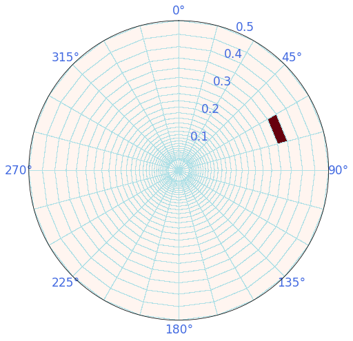
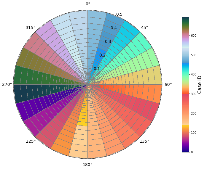
A number of 696 cases need to be run, corresponding to all the combinations of the spectra disctretized in 24 directions and 29 frequencies.
Below is an example of one of the monochromatic cases, with a freq ~0.3 (T = 3.3s) and Dir = 75

Plot_grid_cells(sp, pos=[25, 12]);

Obtain the parameters of the monochromatic cases

# each SWAN case is defined by 5 wave parameters: hs, tp, dir, spr, gamma
vns = ['hs','per','dir','spr','gamma']

gamma = 50  # waves gamma 
spr = 3     # waves directional spread

# initialize case variables
cases = np.full([len(sp.freq) * len(sp.dir), len(vns)], np.nan)
cases_id = np.full([len(sp.freq), len(sp.dir)], np.nan)

c = 0  # case counter

# generate one case for each superpoint direction and frequency values
for ix_d, d in enumerate(sp.dir.values):
    for ix_f, f in enumerate(sp.freq.values):
        
        # hs switch
        if 1 / f > 5:
            hs = 1
        else:
            hs = 0.1
       
        # set case parameters
        cases[c, :] = [hs, np.round(1/f,4), d, spr, gamma] 
        
        # set case ID
        cases_id[ix_f, ix_d] = c
        
        c+=1

# cases DataFrame
df = pd.DataFrame(cases, columns = vns)

# plot cases ID
Plot_grid_cases(sp, cases_id.astype('int'));

SWAN Project#

These are the different steps that need to be followed to run SWAN:

Create project
Define bathymetry and parameters
Define simulation parameters
Build cases
Run cases

Create project

name = 'binwaves'
sp = SwanProject(p_swan, name)

if not op.isdir(op.join(p_swan, name)):
    os.makedirs(op.join(p_swan, name))

Load bathymetry and its parameters

swan_grid = pk.load(open(p_grid_param, "rb"))
swan_depth = pk.load(open(p_grid_depth, "rb"))

Define bathymetry

# generate project main mesh
main_mesh = SwanMesh()

# bathymetry grid description
main_mesh.dg = swan_grid

# bathymetry depth
main_mesh.depth = swan_depth

# computational grid description
main_mesh.cg = main_mesh.dg.copy()

# set project main mesh
sp.set_main_mesh(main_mesh)

Define SWAN cases

input_params = {
    'set_level': 0,
    'set_convention': 'NAUTICAL',

    'coords_mode': 'SPHERICAL',
    'coords_projection': 'CCM',
    
    'boundw_jonswap': gamma,
    'boundw_period': 'PEAK',

    'boundn_mode': 'CLOSED',
    
    'wind': False,
    'only_wind': False,

    'physics': [
        'FRICTION JONSWAP',
        'BREAKING',
    ],

    'numerics':[
        'OFF QUAD',
    ],
    
    'output_variables': [
        'HSIGN', 'TM02', 'DIR', 'TPS', 'DSPR', 
        'PTHSIGN', 'PTRTP', 'PTDIR', 'PTDSPR', 
    ],
    
    'output_variables_points': [
        'HSIGN', 'TM02', 'DIR', 'TPS', 'DSPR', 
        'PTHSIGN', 'PTRTP', 'PTDIR', 'PTDSPR', 
    ],
}

sp.set_params(input_params)

main_mesh.dg

{'xpc': 184.498816,
 'ypc': -21.57901999999979,
 'alpc': 0,
 'xlenc': 0.7900000000037721,
 'ylenc': 0.977999999999458,
 'mxc': 395,
 'myc': 489,
 'dxinp': 0.0020000000000095497,
 'dyinp': 0.0019999999999988916}

sp.params

{'set_level': 0,
 'set_maxerr': None,
 'set_cdcap': None,
 'set_convention': 'NAUTICAL',
 'coords_mode': 'SPHERICAL',
 'coords_projection': 'CCM',
 'cgrid_mdc': 72,
 'cgrid_flow': 0.03,
 'cgrid_fhigh': 1.0,
 'boundw_jonswap': 50,
 'boundw_period': 'PEAK',
 'boundn_mode': 'CLOSED',
 'physics': ['FRICTION JONSWAP', 'BREAKING'],
 'numerics': ['OFF QUAD'],
 'wind_deltinp': None,
 'level_deltinp': None,
 'compute_deltc': None,
 'output_deltt': None,
 'output_variables': ['HSIGN',
  'TM02',
  'DIR',
  'TPS',
  'DSPR',
  'PTHSIGN',
  'PTRTP',
  'PTDIR',
  'PTDSPR'],
 'output_time_ini_specout': None,
 'output_time_ini_block': None,
 'output_time_ini_table': None,
 'output_points_x': [],
 'output_points_y': [],
 'output_variables_points': ['HSIGN',
  'TM02',
  'DIR',
  'TPS',
  'DSPR',
  'PTHSIGN',
  'PTRTP',
  'PTDIR',
  'PTDSPR'],
 'output_spec_deltt': None,
 'output_spec': False,
 'output_points_spec': False,
 'wind': False,
 'only_wind': False}

Swan wrap

sw = SwanWrap_STAT(sp)

Build and launch cases

subset = df.to_xarray().rename({'index':'case'})

# store a copy of the subset
subset.to_netcdf(p_swan_subset)

# store SWAN input spectra for later use
sp_input = np.full([len(subset.case), len(freqs), len(dirs)], 0.0)

for case in subset.case:
    inp = subset.sel(case = case)
    k = 1.1
    f = 1/inp.per.values
    d = inp.dir.values
    i = np.argmin(np.abs(freqs-f))
    j = np.argmin(np.abs(dirs-d))
    
    sp_input[case, i, j] = k 
    
input_spec = xr.Dataset(
    {
        'hs': (['case','freq','dir'], sp_input),
    }, 
    coords = {
        'case': subset.case, 
        'dir': dirs, 
        'freq': freqs
    }
)

input_spec.to_netcdf(p_swan_input_spec)

if launch_swan:
    
    # build and launch swan cases 
    sw.build_cases(df)
    sw.run_cases()

Data extraction#

Once the SWAN propagations have been run, we have to extract the results in the different points of the grid

# extract swan cases output
memory_safe = True

if memory_safe:

    # This output extraction uses cases chunks to avoid memory problems
    chunk_size = 100

    # prepare a folder to store the chunks
    p_chunks = op.join(p_swan, name, 'extract_output')
    if not op.isdir(p_chunks): os.makedirs(p_chunks)

    # generate chunks of cases to extract
    slices = [[chunk_size*x, chunk_size*(x+1)] for x in range(int(np.ceil(len(df)/chunk_size)))]
    slices[-1][1] = len(df)

    # extract and store each chunk
    for c_ini, c_end in slices:
        out_chk = sw.extract_output(case_ini=c_ini, case_end=c_end) 
        out_chk.to_netcdf(op.join(p_chunks, 'output_chunk_{0}_{1}.nc'.format(c_ini, c_end)))

    # combine all chunks into one output file
    out_sea_mm_sim = xr.open_mfdataset(op.join(p_chunks, '*.nc'))

    # clean temporal folder
    shutil.rmtree(p_chunks)

else:
    
    # load entire cases output at once
    out_sea_mm_sim = sw.extract_output() 

SWAN output postprocess: fix 0.1 Hs cases and add a partition number counter

# Rescale simulations of hs=0.01 multiplying by 10
pos_01 = np.where(subset['hs'] < 1)[0]

# get base Hs values
Hsig = out_sea_mm_sim.Hsig.values
Hs_part = out_sea_mm_sim.Hs_part.values

# fix Hs values
for c in range(len(out_sea_mm_sim.case)):
    if np.isin(c, pos_01):
        Hsig[c,:,:] = Hsig[c,:,:] * 10
        Hs_part[c,:,:,:] = Hs_part[c,:,:,:] * 10

# override Hsig and Hs_part variables
out_sea_mm_sim['Hsig'] = (('case','lat','lon'), Hsig)
out_sea_mm_sim['Hs_part'] = (('case','partition','lat','lon'), Hs_part)
    
    
# Calculate number of partitions at each location
matrix_count = np.full(np.shape(out_sea_mm_sim.Hs_part), 0.0)
matrix_count[np.where(out_sea_mm_sim.Hs_part > 0)] = 1
cont = np.sum(matrix_count, axis=1)
cont[np.where(cont == 0)] = np.nan

# add counter to SWAN output
out_sea_mm_sim['count_parts'] = (('case','lat','lon'), cont)    
   

Store SWAN output

# store output to netcdf
store_xarray_max_compression(out_sea_mm_sim, p_swan_output)

out_sea_mm_sim = xr.open_dataset(p_swan_output)

print(out_sea_mm_sim)

<xarray.Dataset>
Dimensions:      (case: 696, lat: 489, lon: 395, partition: 10)
Coordinates:
  * lon          (lon) float64 184.5 184.5 184.5 184.5 ... 185.3 185.3 185.3
  * lat          (lat) float64 -21.58 -21.58 -21.58 ... -20.61 -20.61 -20.6
  * case         (case) int64 0 1 2 3 4 5 6 7 ... 689 690 691 692 693 694 695
Dimensions without coordinates: partition
Data variables:
    Dir          (case, lat, lon) float32 ...
    Hsig         (case, lat, lon) float32 ...
    Tp           (case, lat, lon) float32 ...
    Tm02         (case, lat, lon) float32 ...
    Dspr         (case, lat, lon) float32 ...
    Hs_part      (case, partition, lat, lon) float32 ...
    Tp_part      (case, partition, lat, lon) float32 ...
    Dir_part     (case, partition, lat, lon) float32 ...
    Dspr_part    (case, partition, lat, lon) float32 ...
    count_parts  (case, lat, lon) float64 ...

Plotting#

Individual cases#

Note

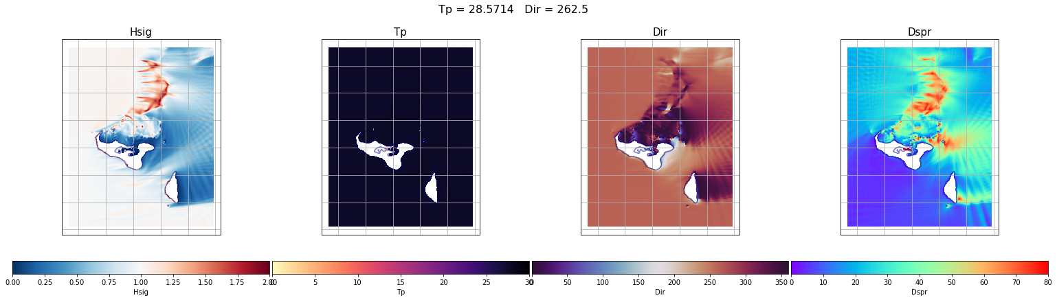
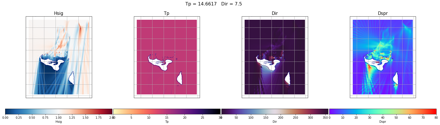
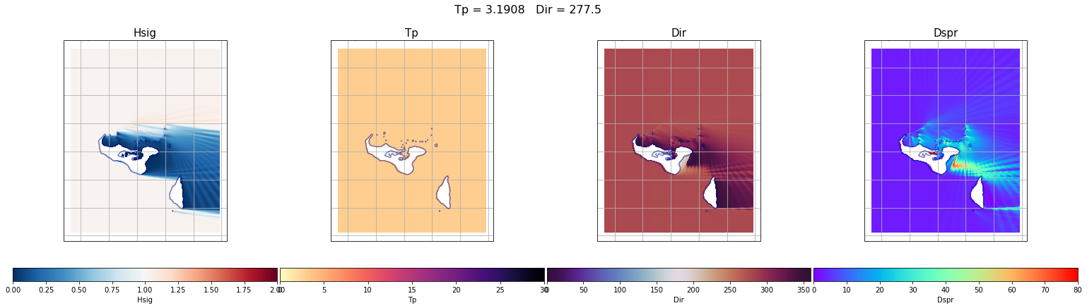
Once the cases have been run and outputs have been extracted, here we plot some results.
First, some individual cases have been plot. From left to right the different variables are: Hs (which corresponds to the propagation coefficient Kp, since we are running unitary wave heights), Tp, Dir and Dspr for the bulk parameters of the simulation, although partitions will be used to determine the propagation coefficients for each case.

case = 0 
lon_s = 184
lat_s = -21

Plot_swan_case(out_sea_mm_sim, subset, case);

case = 500
lon_s = 184
lat_s = -21

Plot_swan_case(out_sea_mm_sim, subset, case);

case = 690
lon_s = 184
lat_s = -21

Plot_swan_case(out_sea_mm_sim, subset, case);

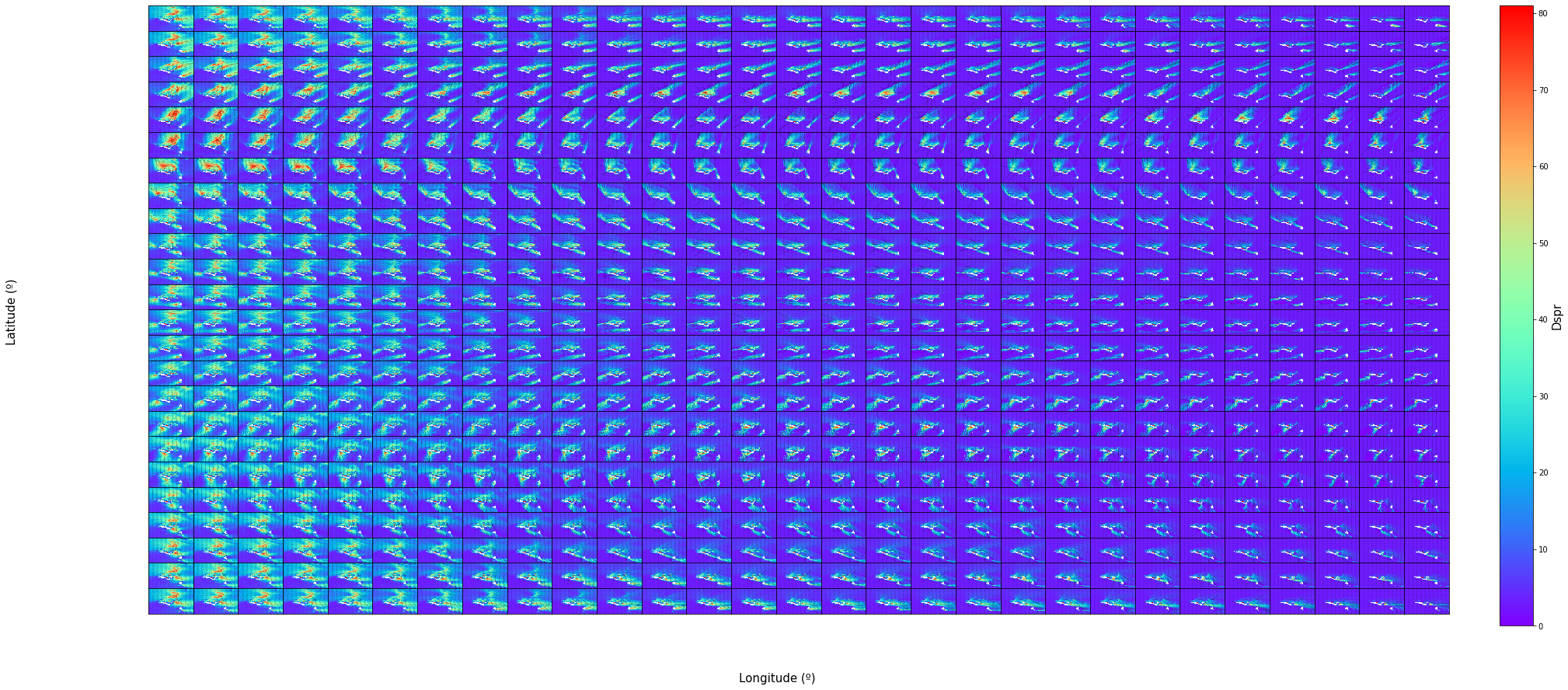
All cases#

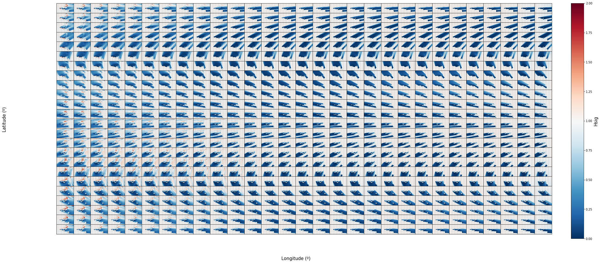
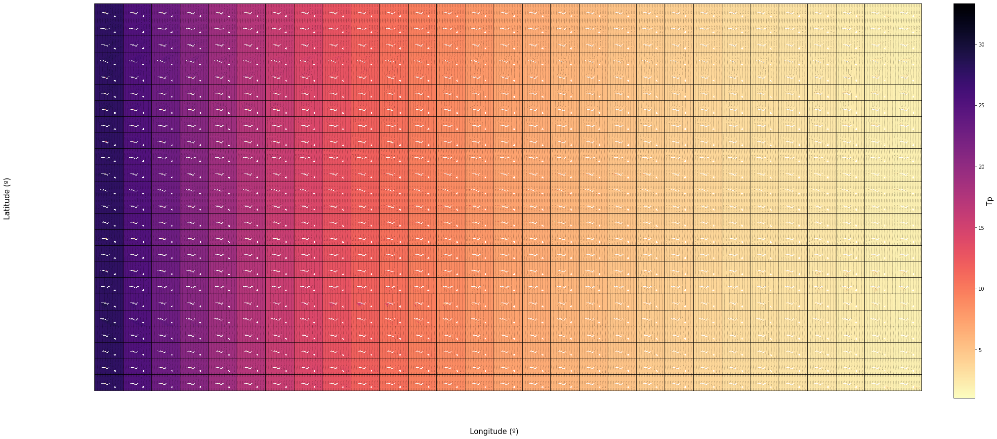
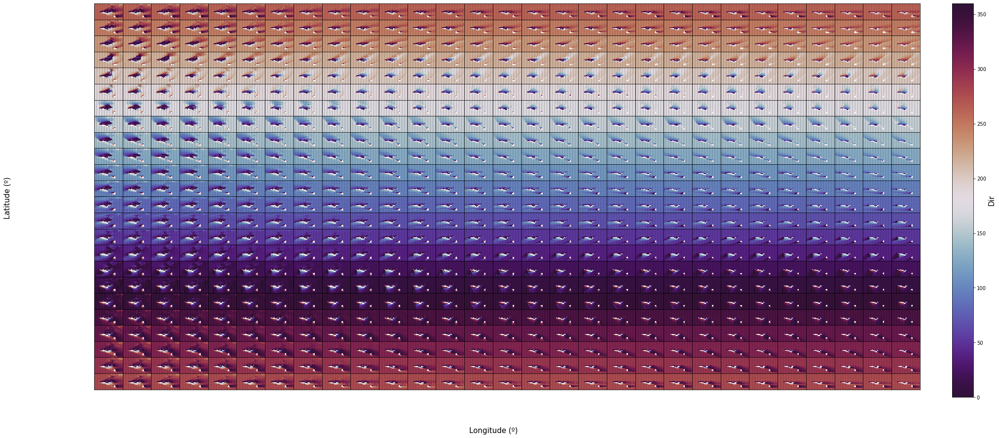
Note

The grids bellow contain the same results but for all of the 696 cases ordered by Dir in rows and Tp in columns.

Hsig

nc = 29
nr = 24
n_cases = nc * nr
vars_ = ['Hsig']

scatter_maps(
    out_sea_mm_sim, 
    n_cases = n_cases,
    n_cols = nc, n_rows = nr,
    var_list = vars_, 
    figsize = [30, 0.6 * nr],
    var_limits = {'Hsig': (0, 2)},
);

TPsmoo

nc = 29
nr = 24
n_cases = nc * nr
vars_ = ['Tp']

scatter_maps(
    out_sea_mm_sim,
    n_cases = n_cases, 
    n_cols = nc, n_rows = nr, 
    var_list = vars_,
    figsize = [30, 0.6 * nr],
);

Dir

nc = 29
nr = 24
n_cases = nc * nr
vars_ = ['Dir']

scatter_maps(
    out_sea_mm_sim,
    n_cases = n_cases,
    n_cols = nc, n_rows = nr,
    var_list = vars_,
    figsize = [30, 0.6 * nr],
);

Dspr

nc = 29
nr = 24
n_cases = nc * nr
vars_ = ['Dspr']

scatter_maps(
    out_sea_mm_sim,
    n_cases = n_cases,
    n_cols = nc, n_rows = nr,
    var_list = vars_,
    figsize  = [30, 0.6 * nr],
);

BinWaves & SWAN

Contents

BinWaves & SWAN#

Methodology#

Database and site parameters#

SWAN Project#

Data extraction#

Plotting#

Individual cases#

All cases#