Waves Hindcast
Contents
Waves Hindcast#
# common
import warnings
warnings.filterwarnings('ignore')
import os
import os.path as op
import sys
import pickle as pk
import time
import datetime

# pip
import xarray as xr
import numpy as np
import pandas as pd
import matplotlib.pyplot as plt

# DEV: bluemath
sys.path.insert(0, op.join(op.abspath(''), '..', '..', '..', '..'))

# bluemath modules
from bluemath.binwaves.reconstruction import reconstruct_kmeans_clusters_hindcast, obtain_wave_metrics_grid
from bluemath.binwaves.reconstruction import get_hindcast_snapshot
from bluemath.binwaves.nino34 import n34_format

from bluemath.binwaves.plotting.hindcast import Plot_hindcast_series_point, Plot_hindcast_snapshot, Plot_hindcast_maps
from bluemath.binwaves.plotting.hindcast import Plot_hindcast_seasonality, Plot_hindcast_elnino
from bluemath.binwaves.plotting.nino34 import Plot_n34
Warning: cannot import cf-json, install "metocean" dependencies for full functionality
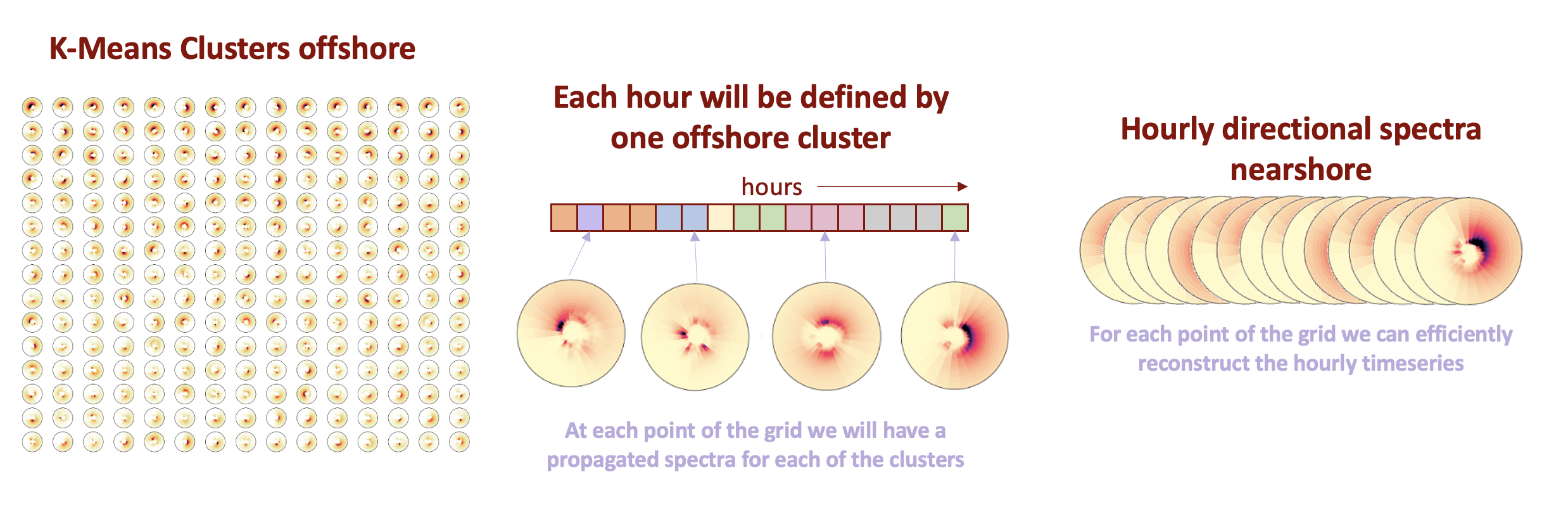
Methodology#
Hindcast
Once we have reconstructed the K-Means clusters for the KMA clusters, and validated the results against instrumental data, we can efficiently reconstruct the hindcast following the steps below
Database and site parameters#
# database
p_data = r'/media/administrador/HD2/SamoaTonga/data'
site = 'Tongatapu'
p_site = op.join(p_data, site)

# deliverable folder
p_deliv = op.join(p_site, 'd05_swell_inundation_forecast')

p_kma = op.join(p_deliv, 'kma')
p_swan = op.join(p_deliv, 'swan')

# nino34 dataset
p_n34 = op.join(p_data, 'ninho34.txt')

# SWAN simulation parameters
name = 'binwaves'
p_swan_subset = op.join(p_swan, name, 'subset.nc')
p_swan_output = op.join(p_swan, name, 'out_main_binwaves.nc')
p_swan_input_spec = op.join(p_swan, name, 'input_spec.nc')

# SuperPoint KMeans
num_clusters = 2000
p_superpoint_kma = op.join(p_kma, 'Spec_KMA_{0}_NS.nc'.format(num_clusters))


# output files
p_site_out = op.join(p_deliv, 'reconstruction')

p_reco_hnd = op.join(p_site_out, 'hindcast')                     # hindcast reconstruction folder
p_hindcast_stats = op.join(p_reco_hnd, 'hindcast_stats.nc')      # hindcast reconstruction metrics
p_hindcast_monthly = op.join(p_reco_hnd, 'hindcast_monthly.nc')  # hindcast monthly mean

# hindcast reconstruction
recon_hindcast = False
wave_metrics = True
wave_metrics_perc = [25, 50, 75, 90, 95, 99]

# hindcast snapshot
hindcast_snapshot = True
time_snapshot = '1993-05-12-00:00:00'
# aux functions

def load_hindcast_recon(point, out_sim, p_reco):
    '''
    Load hindcast reconstruction for a choosen point

    point - point to load [lon, lat] (find nearest)
    out_sim - SWAN simulation output
    '''

    # find point
    ilon = np.argmin(np.abs(out_sim.lon.values - point[0]))
    ilat = np.argmin(np.abs(out_sim.lat.values - point[1]))

    # load coefficient
    fn = 'reconst_hind_lon_{0}_lat_{1}.nc'.format(out_sim.lon.values[ilon], out_sim.lat.values[ilat])
    p_cf = op.join(p_reco, fn)

    return xr.open_dataset(p_cf)
# Load SWAN simulation output and kmeans clusters
out_sim_swan = xr.open_dataset(p_swan_output)
sp_kma = xr.open_dataset(p_superpoint_kma)
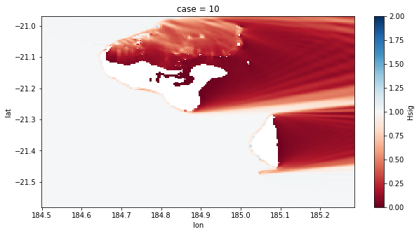
Here we need to define the area for the extraction and the resample factor
The plot is an example of the area that has been cut
# this will reduce memory usage
area_extraction=[184.5, 185.3, -21.62, -20.97]
resample_factor = 2

# cut area
out_sim = out_sim_swan.sel(
    lon = slice(area_extraction[0], area_extraction[1]),
    lat = slice(area_extraction[2], area_extraction[3]),
)

# resample extraction points
out_sim = out_sim.isel(
    lon = np.arange(0, len(out_sim.lon), resample_factor),
    lat = np.arange(0, len(out_sim.lat), resample_factor),
)

# check that the area is OK
plt.figure(figsize = [10, 5])
out_sim.isel(case = 10).Hsig.plot(cmap='RdBu', vmin=0, vmax=2);
Reconstruct Hindcast#
# reconstruct model data for that area
if recon_hindcast:

    reconstruct_kmeans_clusters_hindcast(
        p_site_out, out_sim, sp_kma,
        reconst_hindcast = True,
        override = False,
    )
Obtain wave metrics#
if wave_metrics:

    # calculate wave metrics
    hindcast_stats, hindcast_monthly = obtain_wave_metrics_grid(
        p_reco_hnd,
        out_sim,
        perc = wave_metrics_perc,
    )

    # store metrics and monthly mean
    hindcast_stats.to_netcdf(p_hindcast_stats)
    hindcast_monthly.to_netcdf(p_hindcast_monthly)

else:

    # load metrics and monthly mean
    hindcast_stats = xr.open_dataset(p_hindcast_stats)
    hindcast_monthly = xr.open_dataset(p_hindcast_monthly)
Preprocessing efth and stats...: 100%|██████████████████████████████| 30141/30141 [15:46:10<00:00, 1.88s/it]
hindcast_monthly
<xarray.Dataset>
Dimensions:  (lat: 153, lon: 197, time: 502)
Coordinates:
  * lat      (lat) float64 -21.58 -21.58 -21.57 -21.57 ... -20.98 -20.98 -20.97
  * lon      (lon) float64 184.5 184.5 184.5 184.5 ... 185.3 185.3 185.3 185.3
  * time     (time) datetime64[ns] 1979-01-31 1979-02-28 ... 2020-10-31
Data variables:
    hs       (lon, lat, time) float64 1.857 1.846 1.957 ... 2.079 2.249 1.799
    tp       (lon, lat, time) float64 8.63 12.42 12.14 ... 11.78 10.44 13.16
    tm       (lon, lat, time) float64 6.02 7.039 7.092 ... 6.927 6.476 7.148
    dm       (lon, lat, time) float64 126.0 158.6 134.6 ... 133.1 137.5 178.6
    dp       (lon, lat, time) float64 155.0 194.7 183.7 ... 165.0 184.2 217.5
    dspr     (lon, lat, time) float64 52.32 59.18 58.27 ... 50.72 49.67 62.21
xarray.Dataset
- lat: 153
- lon: 197
- time: 502
- lat(lat)float64-21.58 -21.58 ... -20.98 -20.97
array([-21.57902, -21.57502, -21.57102, -21.56702, -21.56302, -21.55902, -21.55502, -21.55102, -21.54702, -21.54302, -21.53902, -21.53502, -21.53102, -21.52702, -21.52302, -21.51902, -21.51502, -21.51102, -21.50702, -21.50302, -21.49902, -21.49502, -21.49102, -21.48702, -21.48302, -21.47902, -21.47502, -21.47102, -21.46702, -21.46302, -21.45902, -21.45502, -21.45102, -21.44702, -21.44302, -21.43902, -21.43502, -21.43102, -21.42702, -21.42302, -21.41902, -21.41502, -21.41102, -21.40702, -21.40302, -21.39902, -21.39502, -21.39102, -21.38702, -21.38302, -21.37902, -21.37502, -21.37102, -21.36702, -21.36302, -21.35902, -21.35502, -21.35102, -21.34702, -21.34302, -21.33902, -21.33502, -21.33102, -21.32702, -21.32302, -21.31902, -21.31502, -21.31102, -21.30702, -21.30302, -21.29902, -21.29502, -21.29102, -21.28702, -21.28302, -21.27902, -21.27502, -21.27102, -21.26702, -21.26302, -21.25902, -21.25502, -21.25102, -21.24702, -21.24302, -21.23902, -21.23502, -21.23102, -21.22702, -21.22302, -21.21902, -21.21502, -21.21102, -21.20702, -21.20302, -21.19902, -21.19502, -21.19102, -21.18702, -21.18302, -21.17902, -21.17502, -21.17102, -21.16702, -21.16302, -21.15902, -21.15502, -21.15102, -21.14702, -21.14302, -21.13902, -21.13502, -21.13102, -21.12702, -21.12302, -21.11902, -21.11502, -21.11102, -21.10702, -21.10302, -21.09902, -21.09502, -21.09102, -21.08702, -21.08302, -21.07902, -21.07502, -21.07102, -21.06702, -21.06302, -21.05902, -21.05502, -21.05102, -21.04702, -21.04302, -21.03902, -21.03502, -21.03102, -21.02702, -21.02302, -21.01902, -21.01502, -21.01102, -21.00702, -21.00302, -20.99902, -20.99502, -20.99102, -20.98702, -20.98302, -20.97902, -20.97502, -20.97102]) - lon(lon)float64184.5 184.5 184.5 ... 185.3 185.3
array([184.500816, 184.504816, 184.508816, 184.512816, 184.516816, 184.520816, 184.524816, 184.528816, 184.532816, 184.536816, 184.540816, 184.544816, 184.548816, 184.552816, 184.556816, 184.560816, 184.564816, 184.568816, 184.572816, 184.576816, 184.580816, 184.584816, 184.588816, 184.592816, 184.596816, 184.600816, 184.604816, 184.608816, 184.612816, 184.616816, 184.620816, 184.624816, 184.628816, 184.632816, 184.636816, 184.640816, 184.644816, 184.648816, 184.652816, 184.656816, 184.660816, 184.664816, 184.668816, 184.672816, 184.676816, 184.680816, 184.684816, 184.688816, 184.692816, 184.696816, 184.700816, 184.704816, 184.708816, 184.712816, 184.716816, 184.720816, 184.724816, 184.728816, 184.732816, 184.736816, 184.740816, 184.744816, 184.748816, 184.752816, 184.756816, 184.760816, 184.764816, 184.768816, 184.772816, 184.776816, 184.780816, 184.784816, 184.788816, 184.792816, 184.796816, 184.800816, 184.804816, 184.808816, 184.812816, 184.816816, 184.820816, 184.824816, 184.828816, 184.832816, 184.836816, 184.840816, 184.844816, 184.848816, 184.852816, 184.856816, 184.860816, 184.864816, 184.868816, 184.872816, 184.876816, 184.880816, 184.884816, 184.888816, 184.892816, 184.896816, 184.900816, 184.904816, 184.908816, 184.912816, 184.916816, 184.920816, 184.924816, 184.928816, 184.932816, 184.936816, 184.940816, 184.944816, 184.948816, 184.952816, 184.956816, 184.960816, 184.964816, 184.968816, 184.972816, 184.976816, 184.980816, 184.984816, 184.988816, 184.992816, 184.996816, 185.000816, 185.004816, 185.008816, 185.012816, 185.016816, 185.020816, 185.024816, 185.028816, 185.032816, 185.036816, 185.040816, 185.044816, 185.048816, 185.052816, 185.056816, 185.060816, 185.064816, 185.068816, 185.072816, 185.076816, 185.080816, 185.084816, 185.088816, 185.092816, 185.096816, 185.100816, 185.104816, 185.108816, 185.112816, 185.116816, 185.120816, 185.124816, 185.128816, 185.132816, 185.136816, 185.140816, 185.144816, 185.148816, 185.152816, 185.156816, 185.160816, 185.164816, 185.168816, 185.172816, 185.176816, 185.180816, 185.184816, 185.188816, 185.192816, 185.196816, 185.200816, 185.204816, 185.208816, 185.212816, 185.216816, 185.220816, 185.224816, 185.228816, 185.232816, 185.236816, 185.240816, 185.244816, 185.248816, 185.252816, 185.256816, 185.260816, 185.264816, 185.268816, 185.272816, 185.276816, 185.280816, 185.284816]) - time(time)datetime64[ns]1979-01-31 ... 2020-10-31
array(['1979-01-31T00:00:00.000000000', '1979-02-28T00:00:00.000000000',
       '1979-03-31T00:00:00.000000000', ..., '2020-08-31T00:00:00.000000000',
       '2020-09-30T00:00:00.000000000', '2020-10-31T00:00:00.000000000'],
      dtype='datetime64[ns]')
- hs(lon, lat, time)float641.857 1.846 1.957 ... 2.249 1.799
array([[[1.85689833, 1.84610125, 1.95653097, ..., 2.17962268, 2.31169969, 2.13923995], [1.8559314 , 1.84596206, 1.9563295 , ..., 2.17868128, 2.31028047, 2.13841993], [1.85419645, 1.84537914, 1.95562912, ..., 2.17761737, 2.30860774, 2.13766966], ..., [1.56519628, 1.79983312, 1.75784129, ..., 2.01177915, 2.13330522, 2.12799962], [1.56930598, 1.80298574, 1.75824014, ..., 2.01534971, 2.13772511, 2.13382285], [1.57255749, 1.80431447, 1.75682696, ..., 2.01782221, 2.14150775, 2.13923604]], [[1.85693773, 1.84560922, 1.95637708, ..., 2.17942027, 2.31177151, 2.13921765], [1.85513441, 1.84509275, 1.95570158, ..., 2.17793271, 2.30961651, 2.13797572], [1.85399312, 1.84486733, 1.9554251 , ..., 2.17689067, 2.30805778, 2.13709116], ... [1.92699048, 1.87641745, 1.97749279, ..., 2.07783672, 2.24765982, 1.80026897], [1.92793734, 1.87916797, 1.97947752, ..., 2.08083308, 2.25113726, 1.80528041], [1.9289832 , 1.88248325, 1.98177134, ..., 2.08642196, 2.25675467, 1.81526715]], [[1.95757925, 1.95696218, 2.03604528, ..., 2.29650751, 2.42101368, 2.22060645], [1.95763409, 1.95615913, 2.03598872, ..., 2.29614712, 2.42046741, 2.22014906], [1.95749251, 1.95501919, 2.03565829, ..., 2.29581337, 2.41994238, 2.21992163], ..., [1.92668669, 1.87449737, 1.97584631, ..., 2.07577527, 2.24441619, 1.79562506], [1.92671179, 1.87553192, 1.97593606, ..., 2.07560551, 2.24546251, 1.794013 ], [1.92712865, 1.8775778 , 1.97692575, ..., 2.07874899, 2.24902836, 1.79865087]]]) - tp(lon, lat, time)float648.63 12.42 12.14 ... 10.44 13.16
array([[[ 8.62995401, 12.42268227, 12.14324475, ..., 12.65098684, 12.0955141 , 13.21149104], [ 8.63106115, 12.41985541, 12.05312812, ..., 12.65115975, 12.09603089, 13.21149637], [ 8.63146204, 12.41861292, 12.145112 , ..., 12.65137867, 12.09656124, 13.21159618], ..., [10.14158547, 12.72827053, 13.73346257, ..., 12.54328092, 12.7074115 , 13.20599749], [10.10853519, 12.73727888, 13.72769642, ..., 12.53908415, 12.56250253, 13.20664075], [10.12886258, 12.7253373 , 13.73639527, ..., 12.52345373, 12.55333323, 13.20642672]], [[ 8.62926385, 12.42336105, 12.14351473, ..., 12.65099568, 12.09475648, 13.21161006], [ 8.63156265, 12.42223898, 12.14336011, ..., 12.65156233, 12.09641057, 13.21134186], [ 8.63222606, 12.41949298, 12.05342733, ..., 12.65169068, 12.09706335, 13.21147906], ... [ 8.57892763, 11.03280209, 10.81160621, ..., 11.69254809, 10.31501808, 13.13005003], [ 8.58161522, 11.04287352, 10.8594535 , ..., 11.77905056, 10.44013876, 13.16654488], [ 8.58269796, 11.08104095, 10.86073407, ..., 11.79037102, 10.44595814, 13.20386478]], [[ 8.64163165, 11.8253805 , 11.02913243, ..., 12.35472035, 11.78573219, 13.20190005], [ 8.64154828, 11.82828177, 11.02923903, ..., 12.35529324, 11.78604115, 13.20165261], [ 8.64180673, 12.01296486, 11.02912766, ..., 12.35575213, 11.78637457, 13.20202101], ..., [ 8.57410031, 11.01836648, 10.81556939, ..., 11.57434908, 10.06315656, 13.09222453], [ 8.57619734, 11.02627521, 10.81166432, ..., 11.65189467, 10.17813084, 13.12424488], [ 8.57688401, 11.02357378, 10.85707351, ..., 11.77672446, 10.43689502, 13.15960411]]]) - tm(lon, lat, time)float646.02 7.039 7.092 ... 6.476 7.148
array([[[6.01976347, 7.0390894 , 7.09181969, ..., 7.45595552, 6.78796195, 7.3631241 ], [6.0214388 , 7.04142549, 7.09446444, ..., 7.45735656, 6.78919382, 7.3633062 ], [6.02054888, 7.04092139, 7.09497139, ..., 7.4568987 , 6.78917019, 7.36254462], ..., [5.80508744, 7.05872034, 6.99438752, ..., 7.3144377 , 6.8849471 , 7.37734703], [5.80540853, 7.05313495, 6.98538243, ..., 7.30856548, 6.88350991, 7.37794134], [5.81498984, 7.05290787, 6.98313401, ..., 7.30903861, 6.8919372 , 7.38030363]], [[6.01924213, 7.03768521, 7.09081571, ..., 7.45524514, 6.78755964, 7.36315299], [6.02178913, 7.0421572 , 7.0952347 , ..., 7.45833117, 6.78969164, 7.3640121 ], [6.02310727, 7.04396704, 7.09762975, ..., 7.45931598, 6.79078554, 7.36390174], ... [5.81803346, 6.63488772, 6.7264279 , ..., 6.91747429, 6.46661552, 7.1125171 ], [5.82074569, 6.64227043, 6.73292068, ..., 6.9287791 , 6.4775163 , 7.14303918], [5.82536773, 6.65251092, 6.74141321, ..., 6.94828751, 6.4951115 , 7.19221677]], [[5.83814845, 6.78633195, 6.81438538, ..., 7.2250464 , 6.65566663, 7.32002164], [5.8391766 , 6.78837677, 6.81629392, ..., 7.22700587, 6.65687031, 7.32297946], [5.83996029, 6.79101449, 6.8184429 , ..., 7.22970376, 6.65848364, 7.32715732], ..., [5.81549052, 6.62733755, 6.7193812 , ..., 6.90742686, 6.45650486, 7.08829008], [5.81596078, 6.63045781, 6.72076528, ..., 6.911503 , 6.46178674, 7.10213871], [5.81913635, 6.63841912, 6.72648634, ..., 6.92704665, 6.47644148, 7.14784042]]]) - dm(lon, lat, time)float64126.0 158.6 134.6 ... 137.5 178.6
array([[[126.00130923, 158.63241424, 134.59138473, ..., 164.21878251, 161.36655024, 210.12593008], [126.0001376 , 158.58243517, 134.58152022, ..., 164.26360676, 161.45316183, 210.1993465 ], [126.02326179, 158.58250918, 134.60290805, ..., 164.31574714, 161.55337105, 210.27176418], ..., [116.07336639, 152.7277977 , 155.93193202, ..., 171.16248397, 167.72334559, 214.29647542], [114.98011416, 151.96689611, 155.67105832, ..., 169.41081709, 166.67717232, 213.93027105], [113.7021181 , 151.41635216, 155.34871109, ..., 167.94812656, 165.53682229, 213.5097787 ]], [[126.00666617, 158.73412333, 134.59768616, ..., 164.24644315, 161.36611 , 210.11046 ], [126.04536563, 158.71848959, 134.60684595, ..., 164.32402782, 161.49604541, 210.2073281 ], [126.04528582, 158.6747402 , 134.59814433, ..., 164.37695448, 161.59388093, 210.28893958], ... [108.38384954, 128.89358695, 114.63703376, ..., 133.0789633 , 137.48340971, 178.968713 ], [108.47348959, 129.18981989, 114.88563764, ..., 133.30565811, 137.75012735, 179.29219208], [108.61552317, 129.63425007, 115.30399412, ..., 133.84242464, 138.21227568, 180.20063213]], [[116.5528017 , 140.96964911, 128.06703146, ..., 151.91813671, 151.95402966, 205.90672347], [116.52227367, 140.93122583, 128.05371121, ..., 151.92601567, 151.98863664, 205.88150585], [116.52775518, 140.92141334, 128.07663115, ..., 151.94098495, 152.04891066, 205.84945999], ..., [108.22125111, 128.55697096, 114.40138982, ..., 132.85425121, 137.17928358, 178.74718063], [108.26695408, 128.68789476, 114.53350768, ..., 132.7675623 , 137.23559512, 178.25612642], [108.37708889, 129.03956941, 114.86883191, ..., 133.06819266, 137.53448355, 178.57393865]]]) - dp(lon, lat, time)float64155.0 194.7 183.7 ... 184.2 217.5
array([[[155. , 194.72139673, 183.69463087, ..., 180.13087248, 190.41262136, 217.5 ], [155. , 194.72139673, 183.69463087, ..., 180.13087248, 190.41262136, 217.5 ], [155. , 194.72139673, 183.69463087, ..., 180.13087248, 190.41262136, 217.5 ], ..., [172.31854839, 193.38410104, 206.44630872, ..., 195.03020134, 195.34327323, 217.5 ], [152.78225806, 193.38410104, 209.82885906, ..., 195.03020134, 194.49029126, 217.5 ], [154.59677419, 200.98439822, 210.09060403, ..., 195.03020134, 194.59431345, 217.5 ]], [[155. , 194.72139673, 183.69463087, ..., 180.13087248, 190.41262136, 217.5 ], [155. , 194.72139673, 183.69463087, ..., 180.13087248, 190.41262136, 217.5 ], [155. , 194.72139673, 183.69463087, ..., 180.13087248, 190.41262136, 217.5 ], ... [144.65725806, 177.18053492, 172.60067114, ..., 163.70134228, 183.90083218, 217.5 ], [144.65725806, 177.71545319, 179.02348993, ..., 164.96979866, 184.19209431, 217.5 ], [144.65725806, 177.71545319, 179.02348993, ..., 166.66107383, 185.56518724, 217.5 ]], [[145.50403226, 187.12109955, 157.13758389, ..., 175.88255034, 190.28779473, 217.5 ], [145.50403226, 187.12109955, 157.13758389, ..., 175.88255034, 190.28779473, 217.5 ], [145.50403226, 187.12109955, 157.13758389, ..., 175.88255034, 190.28779473, 217.5 ], ..., [144.65725806, 176.51188707, 182.26510067, ..., 163.70134228, 183.35991678, 217.5 ], [144.65725806, 177.18053492, 182.26510067, ..., 163.70134228, 183.90083218, 217.5 ], [144.65725806, 177.18053492, 188.68791946, ..., 164.96979866, 184.19209431, 217.5 ]]]) - dspr(lon, lat, time)float6452.32 59.18 58.27 ... 49.67 62.21
array([[[52.31835375, 59.17659584, 58.26991876, ..., 50.65732061,
         49.46981342, 47.3330093 ],
        [52.34433244, 59.22402528, 58.28258591, ..., 50.68209414,
         49.48436797, 47.29423869],
        [52.38411491, 59.25768582, 58.29669137, ..., 50.70813924,
         49.4990103 , 47.25940813],
        ...,
        [62.95437476, 65.10075255, 65.27156101, ..., 57.11929934,
         54.74147772, 50.09381558],
        [62.86560592, 65.11454876, 65.39068244, ..., 57.2249402 ,
         54.93967359, 50.63716748],
        [62.74755161, 65.10992117, 65.51416546, ..., 57.27727774,
         55.13298257, 51.11456147]],

       [[52.31803632, 59.15234008, 58.26355348, ..., 50.63482028,
         49.45300785, 47.31813905],
        [52.35761114, 59.20641121, 58.28282024, ..., 50.65588853,
         49.46543616, 47.25534775],
        [52.38981825, 59.25631591, 58.29798841, ..., 50.68365631,
         49.48166076, 47.21275061],
...
        [50.62010667, 59.01846722, 56.05364659, ..., 50.73032191,
         49.64626029, 62.19565299],
        [50.66847113, 59.0765748 , 56.13226316, ..., 50.76233841,
         49.71597197, 62.03454153],
        [50.70138782, 59.1569196 , 56.18155624, ..., 50.83855809,
         49.83028815, 61.80471872]],

       [[51.83388812, 60.19088312, 56.95558895, ..., 53.56505759,
         51.90384989, 54.15954463],
        [51.84282731, 60.20903567, 56.958657  , ..., 53.55417628,
         51.91031379, 54.16148163],
        [51.83010413, 60.21043506, 56.9384813 , ..., 53.53154124,
         51.90614337, 54.13973231],
        ...,
        [50.58302302, 58.95972574, 56.01398093, ..., 50.77078692,
         49.62973373, 62.43513716],
        [50.57082008, 58.94537414, 55.99645067, ..., 50.70856144,
         49.61531055, 62.38408207],
        [50.56433168, 58.97696305, 55.98158469, ..., 50.71795977,
         49.66743699, 62.20865114]]])
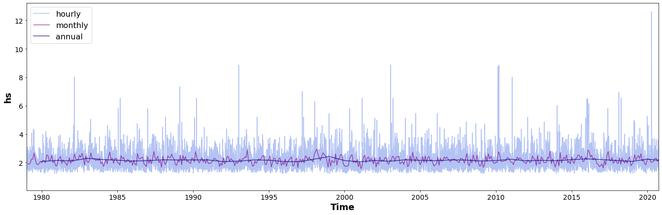
# Plot hindcast at selected point
point = [187.8, -13.88]
# Load hindcast reconstruction at nearest point
recon_data = load_hindcast_recon(point, out_sim, p_reco_hnd)
# monthly hindcast at point
ilon = np.argmin(np.abs(hindcast_monthly.lon.values - point[0]))
ilat = np.argmin(np.abs(hindcast_monthly.lat.values - point[1]))
month_data = hindcast_monthly.isel(lon=ilon, lat=ilat)
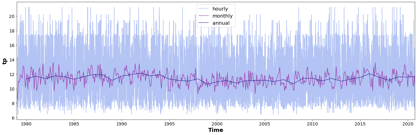
# plot hs, tp and dm time series
Plot_hindcast_series_point(recon_data, month_data, 'hs');
Plot_hindcast_series_point(recon_data, month_data, 'tp');
Plot_hindcast_series_point(recon_data, month_data, 'dm');

Wave climate#
Snapshot analysis#
if hindcast_snapshot:
    data_snapshot = get_hindcast_snapshot(p_reco_hnd, out_sim, time_snapshot)

    # plot hindcast snapshot
    Plot_hindcast_snapshot(data_snapshot)
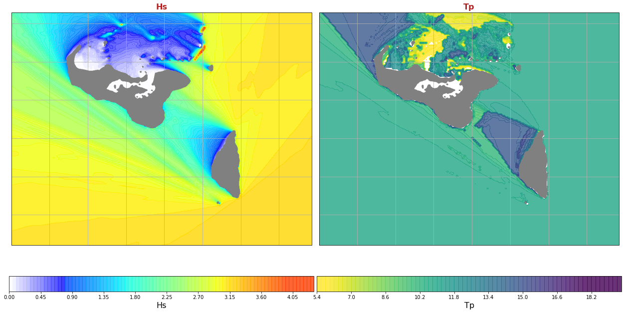
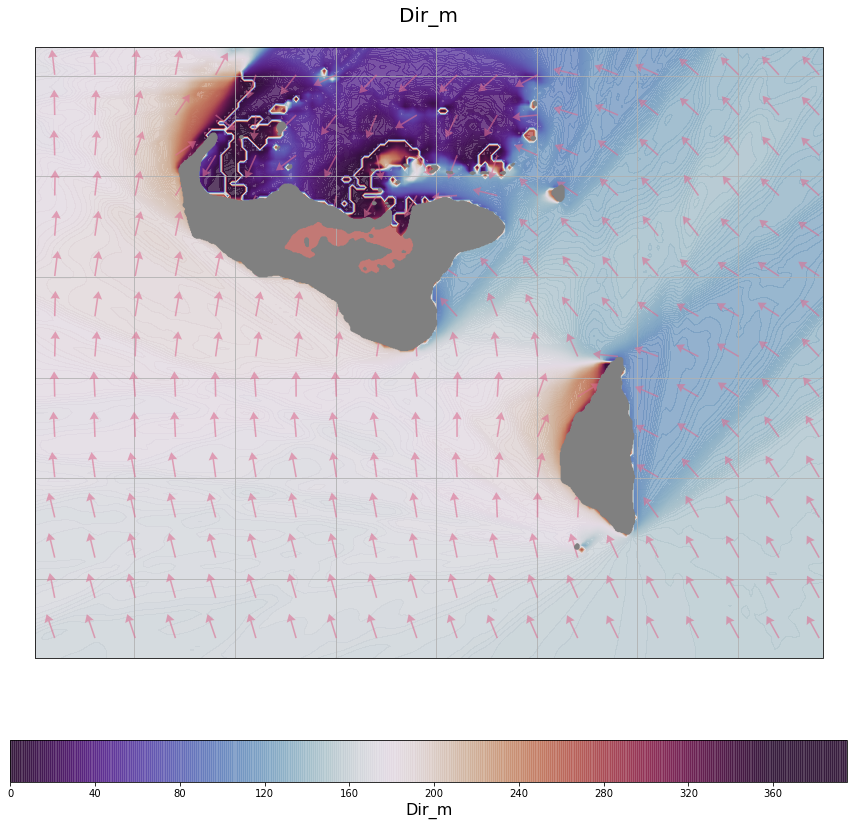
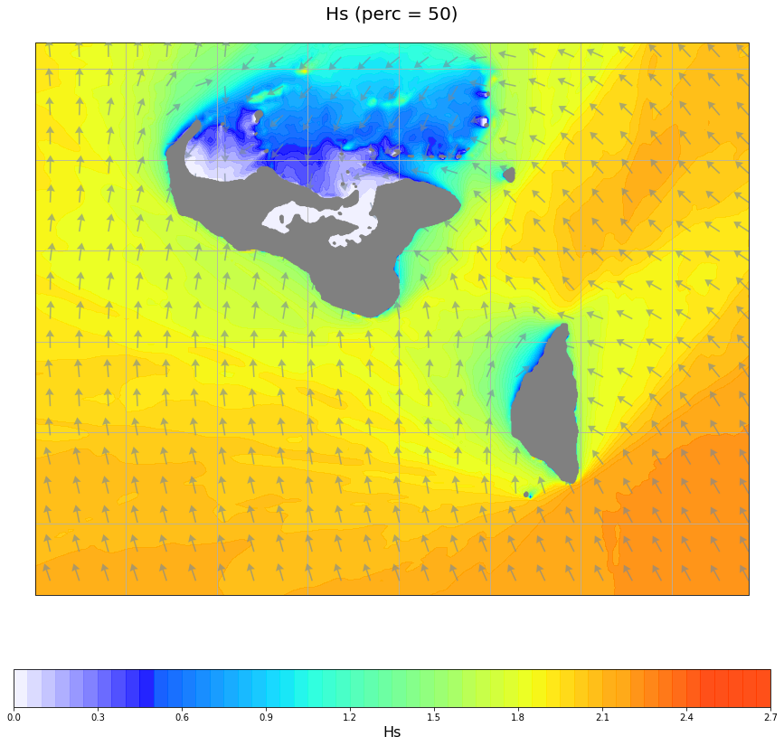
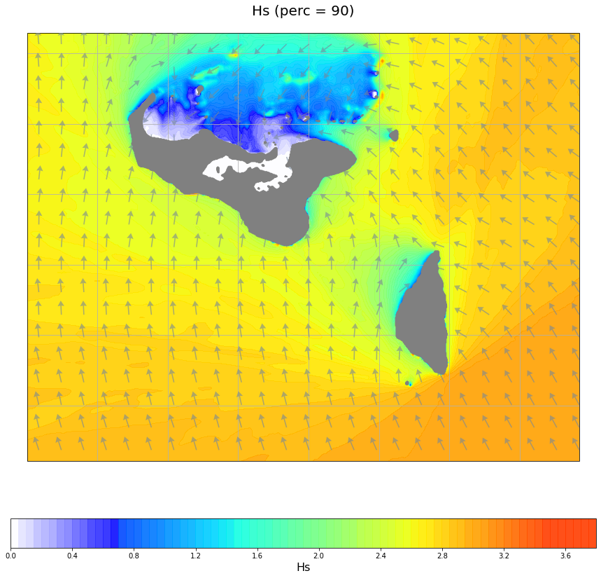
Average climate#
Plot_hindcast_maps(
    hindcast_stats, 'Dir_m',
    vmin = 0, vmax = 360,
    quiv_color = 'palevioletred',
    figsize = [15, 15],
);
Plot_hindcast_maps(
    hindcast_stats, 'Hs',
    percentile = 50,
    vmin = 0, vmax = 2.5,
    quiv_fact = 8, figsize = [15, 15],
);
Plot_hindcast_maps(
    hindcast_stats, 'Hs',
    percentile = 90,
    vmin = 0, vmax = 3.5,
    quiv_fact = 8, figsize = [15, 15],
);
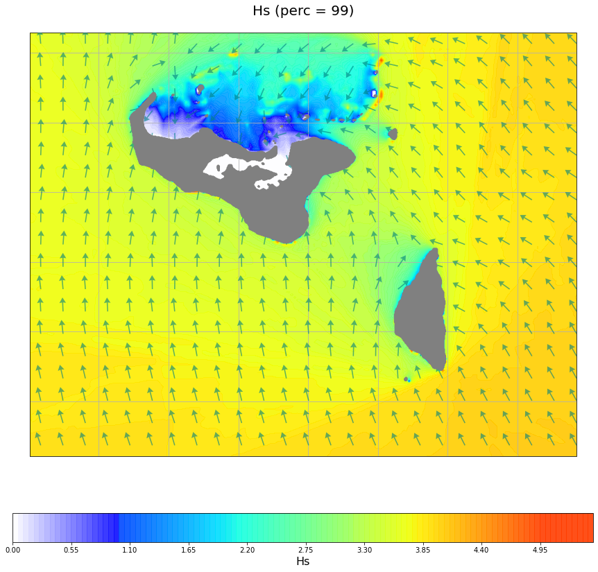
Plot_hindcast_maps(
    hindcast_stats, 'Hs',
    percentile = 99,
    vmin = 0, vmax = 5,
    quiv_fact = 8, quiv_color = 'teal',
    figsize = [15, 15],
);
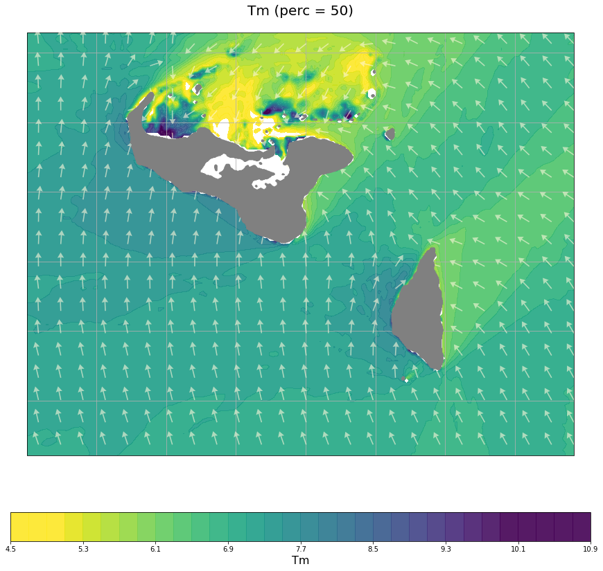
Plot_hindcast_maps(
    hindcast_stats, 'Tm',
    percentile = 50,
    vmin = 5, vmax = 10,
    quiv_fact = 8, quiv_color = 'cornsilk',
    figsize = [15, 15],
);
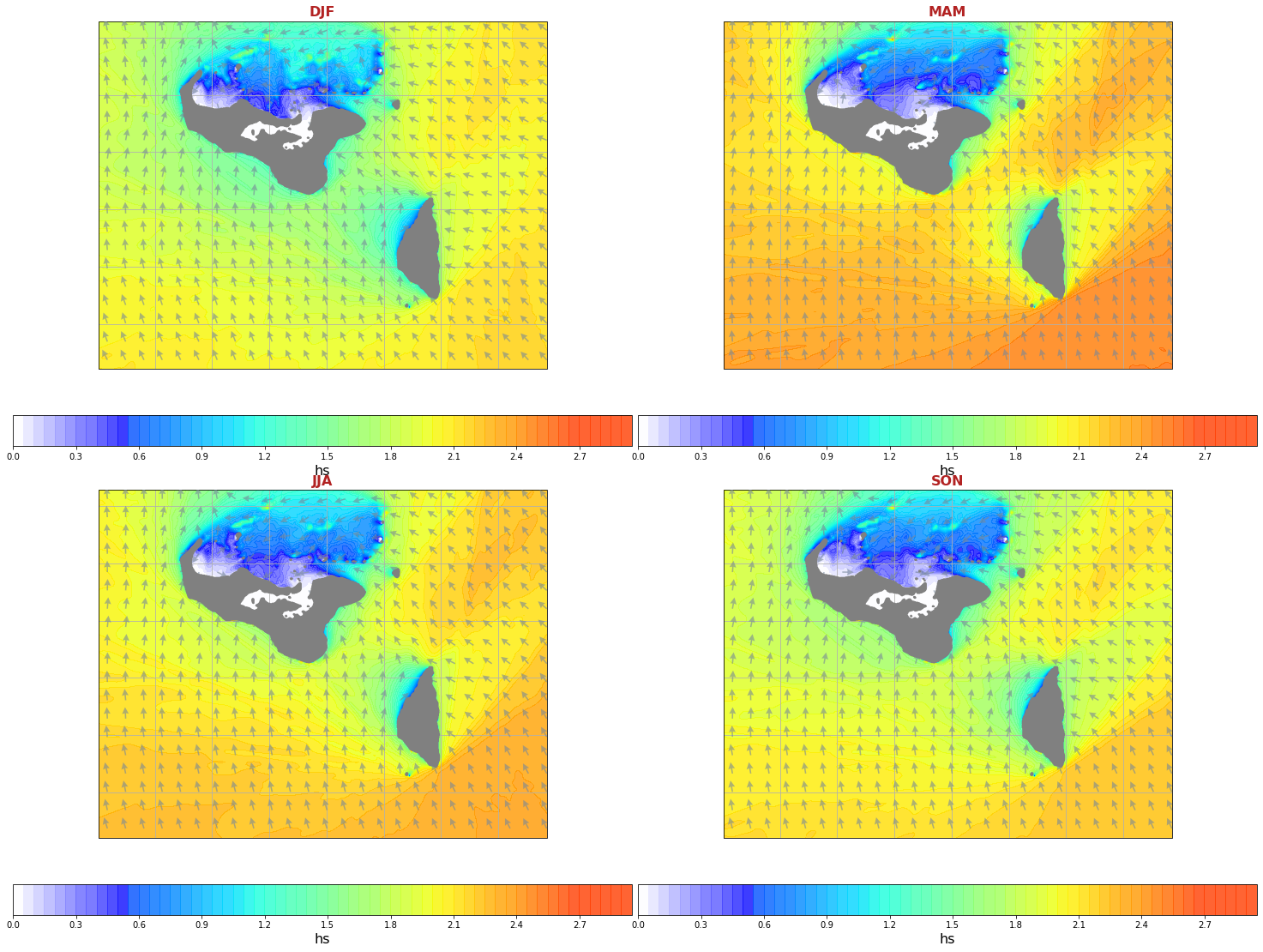
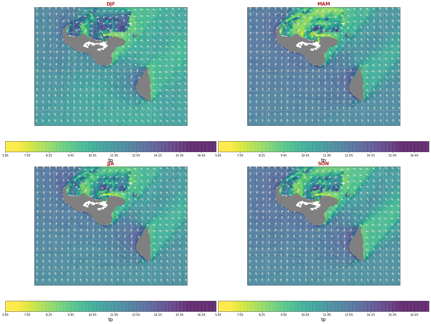
Seasonality#
seasons = hindcast_monthly.groupby('time.season').mean()
Plot_hindcast_seasonality(seasons, var_s = 'hs', vmin = 0, vmax = 2.7);
Plot_hindcast_seasonality(seasons, var_s = 'tm', vmin = 4, vmax = 10, quiv_color = 'cornsilk');
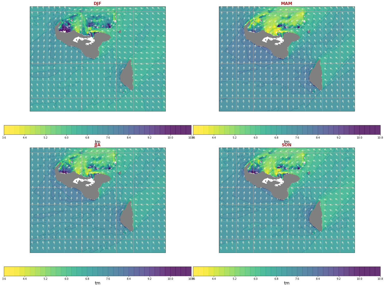
Plot_hindcast_seasonality(seasons, var_s = 'tp', vmin = 6.5, vmax = 16, quiv_color = 'cornsilk');
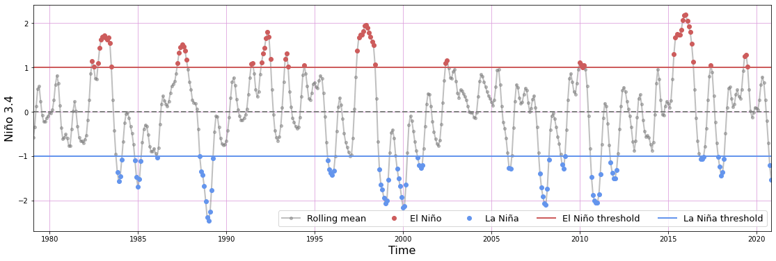
Interannual variability#
# load ninho34 data
n34 = np.loadtxt(p_n34,skiprows=1, max_rows=74)
n34 = n34_format(n34, rolling_mean=True)

n34 = n34.sel(time = hindcast_monthly.time)

# plot ninho34 and thresholds
thr1 = 1   # over this value, years are classified as El Nino (1)
thr2 = -1  # under this value, years are classified as La Nina (3)
Plot_n34(n34, l1 = thr1, l2 = thr2, figsize=[19, 6]);

# add ninho34 classification to monthly hindcast data
hindcast_monthly['n34'] = (('time'), n34.classification.values) # 1:El Nino, 2:Neutral, 3:La Nina
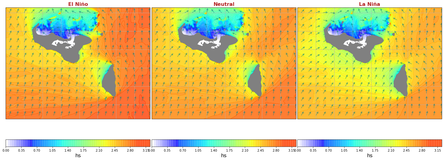
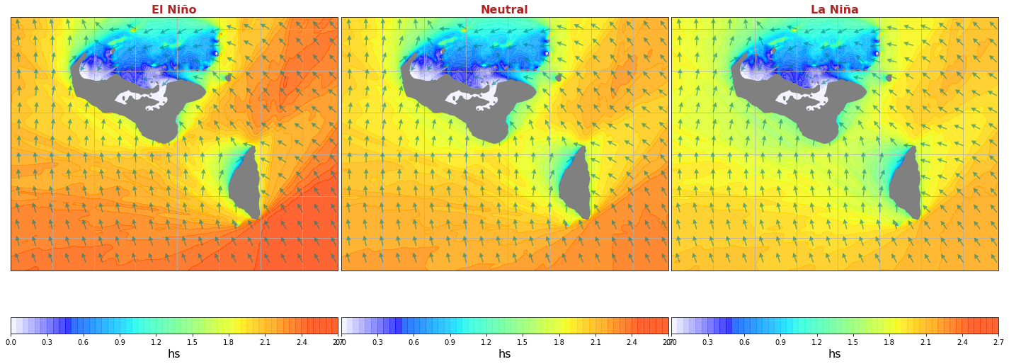
Average waves 50% percentile#
Plot_hindcast_elnino(hindcast_monthly, var_s = 'hs', vmin = 0, vmax = 2.5, figsize=[25,12]);
Extreme waves: 99% percentile#
Plot_hindcast_elnino(hindcast_monthly, quant = 0.99, var_s = 'hs', vmin = 0, vmax = 3, figsize=[25,12]);