Coordinate systems
As the definition of a scalar requires a reference scale (units) to carry out a measurement, to write a vector we need to establish some basic rules over the criteria that we are going to use to define it. These basic rules that we have given ourselves to describe a vector are called coordinate systems.
In this section we will first establish the basic elements that should appear in a coordinate system so that, afterwards, go over the main ones used in physics.
Elements of a coordinate system
When a coordinate system is defined it is necessary to supply the following elements:
Reference point: The point in space that we consider the reference and origin of the coordinate system. This point will be used to measure all vector. Usually it is denoted by the letter \(O\).
Axes: A set of directions, one per dimension of the space in which we are working. On each axis it is necessary indicating the scale employed and it requires an adequate label.
Coordinates: It is important to give instructions to label each point (provide the coordinates) with respect to the origin and axes.
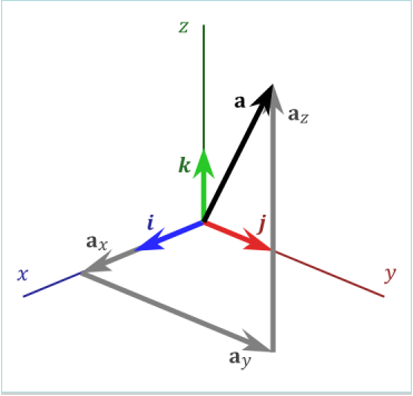
Fig. 2 Three dimensional coordinate system characterized by the axes x, y and z.
Problems and evaluation
The election of the coordinate system is key in the finding the solution of most problems. A good coordinate system will help to find the solution, a bad one will hinder finding it.
In a similar way, the solution to all evaluated problems are expected to have clear indications on the different elections taken by the student in the application of physical laws, how approximations are carried out, etc. Given the large importance of the reference systems in all problems, it is crucial that attention is paid (and explanations given!) to the coordinate system chosen and the reasons behined that election.
Vector basis
It is usual to define a set of vectors along the axis of the coordinate system that have a length of 1 unit along the scale of that axis (as a consequence, this vectors are called unitary).
Cartesian system
A cartesian system is characterized by having orthogonal axes that point in fixed directions (see below for cylindrical or spherical systems where the axes change from point to point) and have well-defined and fixed scales. These are the most usual coordiante systems but are not always present. The axes directions must be defined at the beginning of the problem.
The axes of a cartesian system are usually denoted by the letters \(x\), \(y\), \(z\). In problems where two or more coordinate axes are defined it is usual to use \(x^\prime\), \(x^{\prime\prime}\), \(y^\prime\)… for alternative coordinate system. There are two usual notations for basis vectors, one uses the latin letters i, j, k and the other uses unitary vectors u. Both alternatives and the axes they represent are given in the following table:
Axis |
Vector notation 1 |
Vector notation 2 |
|---|---|---|
x |
\(\vec{i}\) |
\(\vec{u}_x\) |
y |
\(\vec{j}\) |
\(\vec{u}_y\) |
z |
\(\vec{k}\) |
\(\vec{u}_z\) |
Example
In the diagram below a 2-dimensional coordinate system is shown:
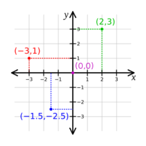
Fig. 3 Two-dimensional coordinate system.
The coordinate system has two cartesian axes x and y aligned with the down-up and left-right directions, respectively. The origin has placed at center of the figure and has coordinates (0,0). An arbitrary point is defined using coordinates (x,y). Positive coordinate x is on the right and negative on the left. Positive coordinate y is upwards while negative is downwards.
Directional cosines
The projections of a vector over a basis are unique. In the case of a cartesian basis a vector \(\vec{A}\) can be written in the following way:
The values \(a_x\), \(a_y\) y \(a_z\) are the coordinates of \(\vec{A}\) in the cartesian basis. The coordinates of a cartesian system are proportional to the cosine of the angles formed by the vector \(\vec{A}\) with each of the cartesian axes. Looking at Fig. Fig. 4 we can see the following relationships:
where \(\vert \vec{A} \vert\) is the modulus of \(\vec{A}\) and takes the value,
The cosines \(\cos\alpha\), \(\cos\beta\) and \(\cos\gamma\) are called directional cosines.
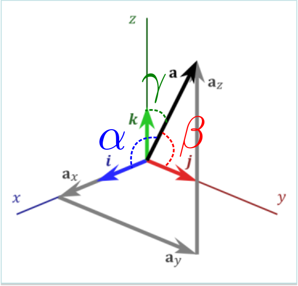
Fig. 4 Three dimensional coordinate sytem showing the angles \(\alpha\), \(\beta\), \(\gamma\) that go into the directional cosines for vector \(\vec{a}\).
Polar system
A polar system is characterized by having two orthogonal axes that are oriented in a different point of space. The points in this system are labelled using two coordinates, the first is the distance of the point to the origin and it is denoted by the greek letter \(\rho\), the second is the angle, from the x-axis in a counter clockwise sense, \(\varphi\). The radial coordinate is a distance and, as such, it is necessarily positive. On the other hand the angle can only take values between 0 and \(2\pi\) although we could also consider larger or smaller values that repeat coordinates in this interval with frequency \(2\pi\).
The axis of a polar system are usually denoted by the greek letters \(\rho\) (radial) and \(\varphi\) (tangential) and the basis vectors are \(\vec{u}_{\rho}\) (radial direction) and \(\vec{u}_{\varphi}\) (tangential direction). Looking at Fig. Fig. 5 one can see that the first axis points radially from the origin while the other is perpendicular to the first and tangent to the circunference centered at the origin and passing through point P.
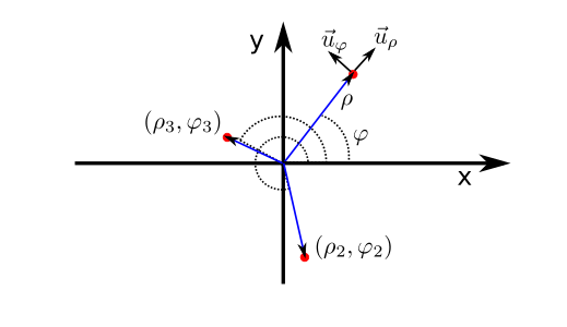
Fig. 5 Bidimensional, polar coordinate system.
Please note that, at difference with the cartesian system where the basis vectors are independent to the point, in this system the basis vectors turn in space. This gives them much flexibility but, at the same time, it is important to be careful with them as, for example, one wishes to calculte the variation of a vector with time in polar coordinates as it will be necessary to taek into account the turning of its basis with position.
In the following two generalization of the polar system to three dimensions, the cylindrical and spherical systems, are described.
Cylindrical system
The cylindrical system is very similar to the polar, as the coordinates \((\rho,\varphi,z)\) correspond with, respectively, with a radial axis and a tangential in the plane like the previous system, extended by a cartesian vector along the third coordinate of space (z axis). The vectors associated to these axes, shown in Fig. Fig. 6, are \(\vec{u}_{\rho}\), \(\vec{u}_{\varphi}\) and \(\vec{u}_{z}\). In this case, \(\rho\) takes values between 0 and infinity, \(\varphi\) between 0 and \(2\pi\) while z changes between \(-\infty\) y \(\infty\).
In the table at the end of the page the transformation from the cylindrical system to the cartesian one is given.
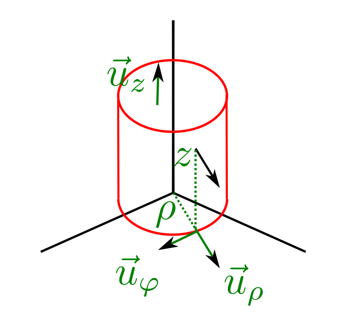
Fig. 6 The cylindrical coordinate system, with its unitary vectors denoted on the surface of a cylinder.
Spherical system
In the spherical system the coordinates of a point are written \((\rho,\theta,\varphi)\) and corresond, respectively, to the distance of the origin to the point (\(\rho\)), an elevation angle (\(\theta\)) that measures the projection of the vector \(\vec{P}\) with the z axis, pointing from the origin to the poles of an imaginary sphere centered on the origin. Finally, the angle \(\varphi\) measures the azimuthal angle, that is to say the orientation of the point when the vector \(\vec{A}\) is projected on the xy-plane. As can be seen on Fig. \(\theta\) can only take values between 0 y \(\pi\) while \(\varphi\) can vary between 0 and \(2\pi\).
In the following table the transformation between the spherical and cylindrical systems to the cartesian one are shown.
System |
Coordinates |
x |
y |
z |
|---|---|---|---|---|
Polar |
\((\rho,\varphi)\) |
\(\rho \cos(\varphi)\) |
\(\rho \sin(\varphi)\) |
\(-\) |
Cylindrical |
\((\rho,\varphi,z)\) |
\(\rho \cos(\varphi)\) |
\(\rho \sin(\varphi)\) |
\(z\) |
Spherical |
\((\rho,\theta,\varphi)\) |
\(\rho \sin(\theta)\cos(\varphi)\) |
\(\rho \sin(\theta)\sin(\varphi)\) |
\(\rho \cos(\theta)\) |