.md .pdf

Contents

Physical Magnitudes

Physics is devoted to the quantitative discusion of nature. In order to do so, it is necessary to define different magnitudes like velocity, acceleration, mass, charge, electromagnetic fields, etc. that, later on, we will use in this description of nature.

A first overall classification of these magnitudes is the one that allows discriminating between scalar and vector magnitudes. It is important to note that this classification is incomplete as there are magnitudes that need to be introducing even more complex mathematical objects like matrixes, although they will not be used during this course. It is also remarkable that, in general, physical laws can be written using tensores that are, in a very simplified sense, lists of numbers in one or more dimensions that transform in a very specific way between different coordinate systems.

Within the definition of magnitudes, the concepts of unit (Sec. Magnitudes escalares), scientific notation (Sec. Scientific notation) and measurement error (Sec. Error of a magnitude) are very important and will be discussed in each of the subsections below.

Magnitudes escalares

A scalar magnitude is defined just by its value that will take, in most cases, the form of a real number and the units in which the value is expressed. This value does not have a priviledged or special direction and it is the same in all directions.

Notation: Each of these magnitudes can be denoted by a capital or lowercase letter of the latin or greek alphabets.

Examples

Some examples of scalar magnitudes, with their usual units are:

• Mass (m, unit: Kg): This kid’s mass is 17 Kg.

• Height (h, unidad: m): This kid is 1.2 m tall.

• Área (A o S, unit: m\(^2\)): This wood has an area of \(2\cdot10^4 m^2\).

• Panthers per forest (unit: panthers/forest): In this forest there are 3 panthers so that the density is 3 panthers/forest.

Vector magnitudes

A vector magnitude is defined by the origin of the vector, its direction (the imaginary line along which the vector is placed), its sense (the direction in which the line is traced) and its magnitude (how long the vector is along the line, given in some particular units).

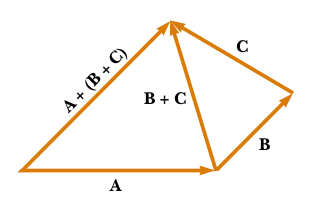
Fig. 1 This image shows different vectors \(\vec{A}\), \(\vec{B}\) and \(\vec{C}\) whose modulus, origin and direction are different. These vectors can be combined in different ways as shown by its sums.

Notation: These magnitudes can be denoted by a capital or lowercase letter of the latin or greek alphabets topped by a small arrow. In some texts, instead of an arrow the magnitude is written in a bold font.

Examples

Some examples of vector magnitudes are:

• Position (\(\vec{r}\), unit: m): My house is 100m west and 50m north of the townhall (origin).

• Velocity (\(\vec{v}\), unit: m/s): The car moves at a velocity of \(\vec{v}=100.0\vec{i}+20.0\vec{j} (Km/h)\)

• Electric field (\(\vec{E}\), unit: V/m): The electric field goes from one plate to the other and has an intensity of 0.1 V/m.

Unidades

Except a few magnitudes that are merely mathematical like, for example the numbers \(e\) or \(\pi\), the values that can be measured require the specification of a scale to which the measurement can be compared to. A unit is, precisely, the definition of one of these arbitrary scales that has been agreed upon by the physical community to express that magnitude. Given that without units the scale over which a magnitude is communicated is not defined it is necessary to always provide units when expressing physical values.

There are many international unit systems that constitute sets of units defined in a coherent way and that, usually, are designed to facilitate work in a particular area. Such an example are the atomic units. Some unit systems, like the imperial system have been used by English-speaking countries. Others like the Gaussian system or Gaussian-cgs (centimeter-gram-second) is particularly useful when working in electromagnetism. The dominant system, that is used almost universally, is called international unit system that evolved out of the metric system. This will be the unit system employed along this course.

The international system uses 7 basic magnitudes to define the units of any other physical quantity. It is important to note that other unit systems may opt to choose other basic magnitudes to be defined (and they do!). In the international system we have:

• Time: Seconds (s)

• Length: Metros (m)

• Mass: Kilogram (kg)

• Electric current: Ampere (A)

• Temperature: Kelvin o Kelvin degree (K)

• Mass quantity: Mole (mol)

• Luminous intensity: Candela (cd)

From this basic magnitudes we can obtain derived magnitudes like, for example, velocity, that is measured in \(m/s\), force, that is measured in \(kg\cdot m/s^2\) or charge that is measured in \(A\cdot s\). To avoid hassle, it is usual to define derived units like the Newton that is 1 unit of force in the international system and equals 1 \(kg\cdot m/s^2\). Some of the most usual units in the international system are presented in the following table.

Magnitude	Unit name	Symbol	Value
Force	Newton	N	\(kg\cdot m/s^2\)
Energy	Joule	J	\(kg\cdot m^2/s^2\)
Power	Watt	W	\(kg\cdot m^2/s^3\)

Scientific notation

Given that science is applied to all phenomena in the universe, from those at very large scales to the really tiny ones, it is important to adapt the way in which values are written to a convenient form. For that reason it usual to use the notation \(\pm n.m \times 10^l\) where n is an integer number between 1 and 9, m a positive integer (this time without restrictions in the number of digits) and l yet another integer that can be positive or negative. This writing style is called normalized scientific notation. There exists another scientific notation in engineering where n takes a value between 1 y 999 and \(l\) is multiple of 3. In this course we will use normalized scientific notation. Please note that a dot is used to define the decimal part (not a comma nor an apostrophe) and there is no special notation for thousands, millions, etc.

Examples

Some examples of numbers in scientific notation are:

Value	Normalized scientific notation	Engineering scientific notation
1.0	1.0 o 1.0 \(\times 10^0\)	1.0 o 1.0 \(\times 10^0\)
657.3	6.573 \(\times 10^2\)	657.3 o 657 \(\times 10^0\)
0.00071	7.1 \(\times 10^{-4}\)	710 \(\times 10^{-6}\)
1573000	1.573 \(\times 10^{6}\)	1.573 \(\times 10^6\)

Error of a magnitude

Knowledge of a physical magnitude is always limited by the precision of the machinery used to measure it. If, for example, a scale has a precision of 0.1kg it does not make sense that we express the mass of a melon that we have just bought as 1.7345kg. Thus, the logical way to operate is to limit the number of decimals to the precision of the measurement and indicate that the mass of the melon is 1.7kg or, if we want to give the error in an explicit way, to indicate that the mass is \(1.7\pm 0.1 kg\).

Error of a derived magnitude

In order to see how the error in measurement affects quantities that we do not directly measure but deduct from other measurements we can see how the first vary when the latter change. Let’s imagine first a magnitude A that depends on the quantity \(x\). If we wanted to know the error of A, we could imagine that we substitute in the expression of A a value \(\tilde{x}\) that is not the exact value of x that we will call \(x_E\). If we assume that \(\tilde{x}\) is close to \(x_E\) we can say,

(1)\[A(\tilde{x})=A(\tilde{x}_E)+\left.\frac{dA}{dx}\right\vert_{x_E}(\tilde{x}-x_E)+\cdots\]

Here we can already see that \(\left.\frac{dA}{dx}\right\vert_{x_E}(\tilde{x}-x_E)+\cdots\) measures the error of the measurement. In general, the magnitude that we will accept as measured is not the result of a single attempt at measuring but the average of several (normally many) measurements. Taking averages in the above expression we get,

(2)\[\left\langle A(\tilde{x})\right\rangle=\left\langle A(\tilde{x}_E)+\left.\frac{dA}{dx}\right\vert_{x_E}(\tilde{x}-x_E) \right\rangle = A(\tilde{x}_E)+\left.\frac{dA}{dx}\right\vert_{x_E} \left\langle(\tilde{x}-x_E) \right\rangle=\]

the term \(\left\langle(\tilde{x}-x_E) \right\rangle\) is the error associated to the measurement of \(x\) thus, we can identify the error in \(A\), \(\Delta A\), as the whole last term which takes the value,

(3)\[\Delta A=\left\vert \left.\frac{dA}{dx}\right\vert_{\left\langle x \right\rangle}\right\vert \Delta x\]

In general when A depends on several variables, \(\{x\}_i\), we can extend the previous reasoning so that the error in A is,

(4)\[\Delta A=\sum_i\left\vert \left.\frac{dA}{dx_i}\right\vert_{\{\left\langle x \right\rangle\}}\right\vert \Delta x_i\]

Note that all the terms in the sum above are positive given that all errors are cumulative (having errors in two magnitudes is always worse, raising the total error of the final magnitude, than having it in just one).

Problems and solved examples

Introduction Vectors