Forecast validation
Contents
Forecast validation#
# common
import os
import os.path as op
import sys
import pickle as pk
import pickle5 as pk5

# pip
import numpy as np
import pandas as pd
import xarray as xr

import warnings
warnings.filterwarnings('ignore')

# DEV: bluemath
sys.path.insert(0, op.join(op.abspath(''), '..', '..', '..', '..'))

# bluemath modules
from bluemath.seasonal_forecast_tcs.forecast import process_season_with_file
from bluemath.seasonal_forecast_tcs.ibtracs import ds_timeline

from bluemath.seasonal_forecast_tcs.plotting.forecast import variables_plot_season, Plot_season, \
variables_plot_season_means, Plot_season_means, variables_dwt_forecast_plot, Plot_forecast_dwt, \
variables_plot_forecast, Plot_forecast
Database and site parameters#
# database
p_data = r'/media/administrador/HD2/SamoaTonga/data'
site = 'SamoaTonga'
p_site = op.join(p_data, site)

#reforecast data
path_f = '/media/administrador/HD1/DATABASES/SeasonalForecast_TCs/CFS/forecast_past_data/'

# deliverable
p_deliv = op.join(p_site, 'seasonal_forecast_tcs')

# IBTrACS database
p_ibtracs = op.join(p_data, 'IBTrACS.ALL.v04r00.nc')

#KMA model
p_kma = op.join(p_deliv, 'kma')
p_kma_model = op.join(p_deliv, 'kma', 'kma_index_okb.pkl')

# index predictor values
p_sst_mld_slp_calibration = op.join(p_deliv, 'sst_mld_slp_calibration.nc')
#load data
df = pd.read_pickle(p_deliv+'/df_coordinates_pmin_sst_mld.pkl')
xs = xr.open_dataset(p_sst_mld_slp_calibration)
xds_kma =  xr.open_dataset(p_kma+'/xds_kma_index_vars.nc')
xds_count_tcs_8 = xr.open_dataset(p_deliv+'/xds_count_tcs_8.nc')
xds_count_tcs_8_964 = xr.open_dataset(p_deliv+'/xds_count_tcs_8_964.nc')
xds_timeM = xr.open_dataset(p_deliv+'/xds_timeM.nc')
xds_PCA = xr.open_dataset(p_deliv+'/xds_pca.nc')
# predictor parameters
lo_area = [160, 210]
la_area = [-30, 0]

#lo_SP, la_SP = [130, 250], [-60, 0]
lop1 = 160.25
lop2 = 211
lap1 = -0.25
lap2 = -32
delta = 2
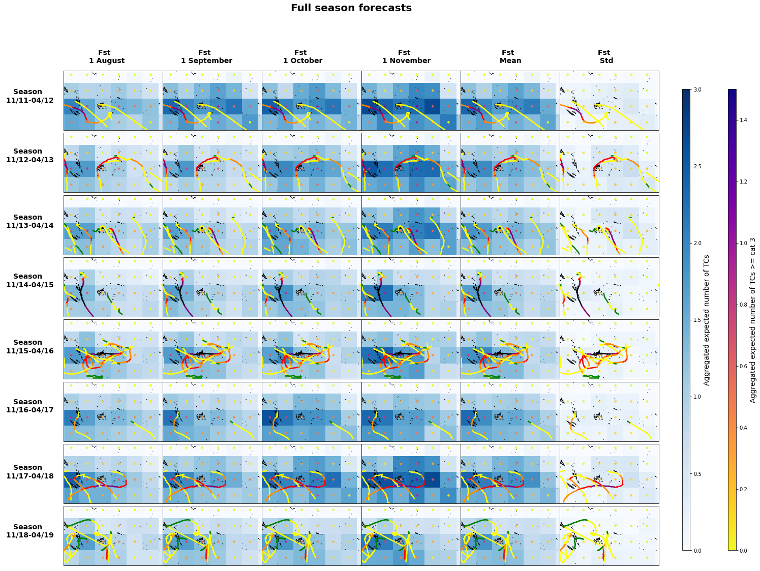
Forecast data validation#
After building and validating the model it will be applied to forecast TCs seasons from previous years to validate this data.
The forecasts from the first day of August, September, October and November. There are four runs per day of the model (00:00,06:00,12:00,18:00 hours).
Steps:
1. Download from CFS 9-month operational forecast and preprocess (file conversion and resolution interpolation) SST and MLD data.
2. Generation of the index predictor based on the index function obtained at the calibration period.
3. The fitted Principal Component Analysis for the calibration is used to predict the index principal components in that same temporal-spatial space.
4. The predicted PCs are assigned to the best match unit group from the fitted K-means clustering -> based on the index predictor a DWT is assigned to each day.
5. From the DWT the expected daily mean number of TCs in 8x8º cells in the target area is known.
Processing season reforecast data#
#2011-2012
path = path_f+'season_11_12/'
y = 2011
process_season_with_file(path,p_kma_model,y,xds_PCA,xds_count_tcs_8 ,xds_count_tcs_8_964,xs, df, lop1, lop2, lap1, lap2, delta)

#2012-2013
path = path_f+'season_12_13/'
y = 2012
process_season_with_file(path,p_kma_model,y,xds_PCA,xds_count_tcs_8 ,xds_count_tcs_8_964,xs, df, lop1, lop2, lap1, lap2, delta)

#2013-2014
path = path_f+'season_13_14/'
y = 2013
process_season_with_file(path,p_kma_model,y,xds_PCA,xds_count_tcs_8 ,xds_count_tcs_8_964,xs, df, lop1, lop2, lap1, lap2, delta)

#2014-2015
path = path_f+'season_14_15/'
y = 2014
process_season_with_file(path,p_kma_model,y,xds_PCA,xds_count_tcs_8 ,xds_count_tcs_8_964,xs, df, lop1, lop2, lap1, lap2, delta)

#2015-2016
path = path_f+'season_15_16/'
y = 2015
process_season_with_file(path,p_kma_model,y,xds_PCA,xds_count_tcs_8 ,xds_count_tcs_8_964,xs, df, lop1, lop2, lap1, lap2, delta)

#2016-2017
path = path_f+'season_16_17/'
y = 2016
process_season_with_file(path,p_kma_model,y,xds_PCA,xds_count_tcs_8 ,xds_count_tcs_8_964,xs, df, lop1, lop2, lap1, lap2, delta)

#2017-2018
path = path_f+'season_17_18/'
y = 2017
process_season_with_file(path,p_kma_model,y,xds_PCA,xds_count_tcs_8 ,xds_count_tcs_8_964,xs, df, lop1, lop2, lap1, lap2, delta)

#2018-2019
path = path_f+'season_18_19/'
y = 2018
process_season_with_file(path,p_kma_model,y,xds_PCA,xds_count_tcs_8 ,xds_count_tcs_8_964,xs, df, lop1, lop2, lap1, lap2, delta)
xds_timeline = ds_timeline(df,xds_count_tcs_8 ,xds_count_tcs_8_964,xds_kma)
print(xds_timeline)
<xarray.Dataset>
Dimensions:         (lat: 5, lon: 8, time: 13879)
Coordinates:
  * time            (time) datetime64[ns] 1982-01-01 1982-01-02 ... 2019-12-31
  * lat             (lat) int64 -30 -22 -14 -6 2
  * lon             (lon) int64 160 168 176 184 192 200 208 216
Data variables:
    bmus            (time) int64 22 22 22 12 25 25 12 ... 18 18 18 23 23 23 18
    mask_tcs        (time) bool False False False False ... True True True True
    id_tcs          (time) object nan nan nan nan ... [13353] [13353] [13353]
    counts_tcs      (time, lat, lon) float64 1.0 nan 2.0 2.0 ... nan nan nan nan
    counts_tcs_964  (time, lat, lon) float64 nan nan 1.0 1.0 ... nan nan nan nan
    probs_tcs       (time, lat, lon) float64 0.003509 nan 0.007018 ... nan nan
    probs_tcs_964   (time, lat, lon) float64 nan nan 0.003509 ... nan nan nan
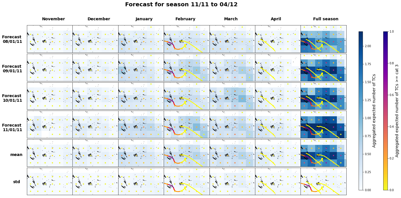
Season reforecast#
2011-12
# TODO: no gestionar asi los output
p_season = path_f+'season_11_12/'
mean_8, mean_8_c3, std_8, std_8_c3, mean_9, \
mean_9_c3, std_9, std_9_c3, mean_10, mean_10_c3, \
std_10, std_10_c3, mean_11,mean_11_c3, std_11, \
std_11_c3, lmean, lmean_c3, lstd, lstd_c3, mean_fs, \
mean_fs_c3, mean_mean, mean_mean_c3, std_mean, \
std_mean_c3, ds4 = variables_plot_season(p_season, 2011, 5, 8)

# TODO: original 5x8 (dx dy)
#std_mean_c3, ds4 = variables_plot_season(p_season_13_14, 2013, 5, 8)
# TODO: xds_timeline??? no lo tengo
Plot_season(
    ds4, 11, 2011, 2.2, 1, mean_8, mean_8_c3,
    std_8, std_8_c3, mean_9, mean_9_c3, std_9,
    std_9_c3, mean_10, mean_10_c3, std_10, std_10_c3,
    mean_11, mean_11_c3, std_11, std_11_c3,
    lmean, lmean_c3, lstd, lstd_c3, mean_fs,
    mean_fs_c3, mean_mean, mean_mean_c3, std_mean,
    std_mean_c3, xds_timeM, 12, df,xds_timeline
);
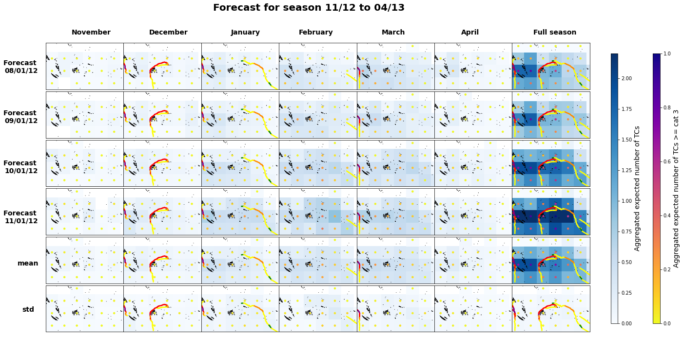
2012-13
# TODO: no gestionar asi los output
p_season = path_f+'season_12_13/'
mean_8, mean_8_c3, std_8, std_8_c3, mean_9, \
mean_9_c3, std_9, std_9_c3, mean_10, mean_10_c3, \
std_10, std_10_c3, mean_11,mean_11_c3, std_11, \
std_11_c3, lmean, lmean_c3, lstd, lstd_c3, mean_fs, \
mean_fs_c3, mean_mean, mean_mean_c3, std_mean, \
std_mean_c3, ds4 = variables_plot_season(p_season, 2012, 5, 8)

# TODO: original 5x8 (dx dy)
#std_mean_c3, ds4 = variables_plot_season(p_season_13_14, 2013, 5, 8)
# TODO: xds_timeline??? no lo tengo
Plot_season(
    ds4, 12, 2012, 2.2, 1, mean_8, mean_8_c3,
    std_8, std_8_c3, mean_9, mean_9_c3, std_9,
    std_9_c3, mean_10, mean_10_c3, std_10, std_10_c3,
    mean_11, mean_11_c3, std_11, std_11_c3,
    lmean, lmean_c3, lstd, lstd_c3, mean_fs,
    mean_fs_c3, mean_mean, mean_mean_c3, std_mean,
    std_mean_c3, xds_timeM, 12, df,xds_timeline
);
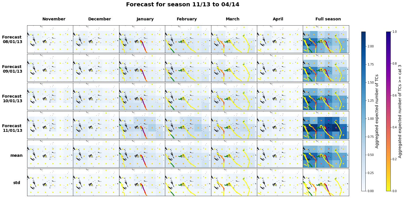
2013-14
# TODO: no gestionar asi los output
p_season = path_f+'season_13_14/'
mean_8, mean_8_c3, std_8, std_8_c3, mean_9, \
mean_9_c3, std_9, std_9_c3, mean_10, mean_10_c3, \
std_10, std_10_c3, mean_11,mean_11_c3, std_11, \
std_11_c3, lmean, lmean_c3, lstd, lstd_c3, mean_fs, \
mean_fs_c3, mean_mean, mean_mean_c3, std_mean, \
std_mean_c3, ds4 = variables_plot_season(p_season, 2013, 5, 8)

# TODO: original 5x8 (dx dy)
#std_mean_c3, ds4 = variables_plot_season(p_season_13_14, 2013, 5, 8)
# TODO: xds_timeline??? no lo tengo
Plot_season(
    ds4, 13, 2013, 2.2, 1, mean_8, mean_8_c3,
    std_8, std_8_c3, mean_9, mean_9_c3, std_9,
    std_9_c3, mean_10, mean_10_c3, std_10, std_10_c3,
    mean_11, mean_11_c3, std_11, std_11_c3,
    lmean, lmean_c3, lstd, lstd_c3, mean_fs,
    mean_fs_c3, mean_mean, mean_mean_c3, std_mean,
    std_mean_c3, xds_timeM, 12, df,xds_timeline
);
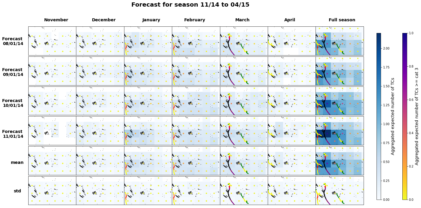
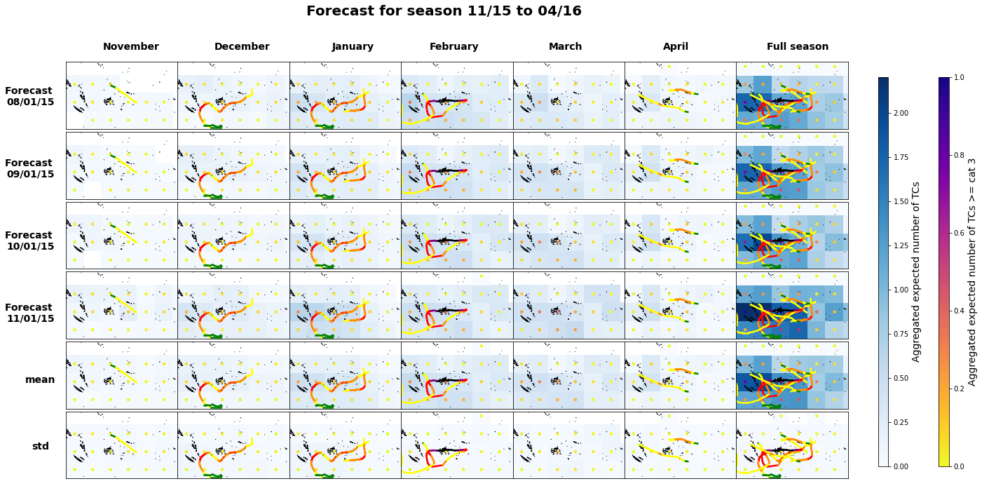
2014-15
# TODO: no gestionar asi los output
p_season = path_f+'season_14_15/'
mean_8, mean_8_c3, std_8, std_8_c3, mean_9, \
mean_9_c3, std_9, std_9_c3, mean_10, mean_10_c3, \
std_10, std_10_c3, mean_11,mean_11_c3, std_11, \
std_11_c3, lmean, lmean_c3, lstd, lstd_c3, mean_fs, \
mean_fs_c3, mean_mean, mean_mean_c3, std_mean, \
std_mean_c3, ds4 = variables_plot_season(p_season, 2014, 5, 8)

# TODO: original 5x8 (dx dy)
#std_mean_c3, ds4 = variables_plot_season(p_season_13_14, 2013, 5, 8)
# TODO: xds_timeline??? no lo tengo
Plot_season(
    ds4, 14, 2014, 2.2, 1, mean_8, mean_8_c3,
    std_8, std_8_c3, mean_9, mean_9_c3, std_9,
    std_9_c3, mean_10, mean_10_c3, std_10, std_10_c3,
    mean_11, mean_11_c3, std_11, std_11_c3,
    lmean, lmean_c3, lstd, lstd_c3, mean_fs,
    mean_fs_c3, mean_mean, mean_mean_c3, std_mean,
    std_mean_c3, xds_timeM, 12, df,xds_timeline
);
2015-2016
# TODO: no gestionar asi los output
p_season = path_f+'season_15_16/'
mean_8, mean_8_c3, std_8, std_8_c3, mean_9, \
mean_9_c3, std_9, std_9_c3, mean_10, mean_10_c3, \
std_10, std_10_c3, mean_11,mean_11_c3, std_11, \
std_11_c3, lmean, lmean_c3, lstd, lstd_c3, mean_fs, \
mean_fs_c3, mean_mean, mean_mean_c3, std_mean, \
std_mean_c3, ds4 = variables_plot_season(p_season, 2015, 5, 8)

# TODO: original 5x8 (dx dy)
#std_mean_c3, ds4 = variables_plot_season(p_season_13_14, 2013, 5, 8)
# TODO: xds_timeline??? no lo tengo
Plot_season(
    ds4, 15, 2015, 2.2, 1, mean_8, mean_8_c3,
    std_8, std_8_c3, mean_9, mean_9_c3, std_9,
    std_9_c3, mean_10, mean_10_c3, std_10, std_10_c3,
    mean_11, mean_11_c3, std_11, std_11_c3,
    lmean, lmean_c3, lstd, lstd_c3, mean_fs,
    mean_fs_c3, mean_mean, mean_mean_c3, std_mean,
    std_mean_c3, xds_timeM, 12, df,xds_timeline
);
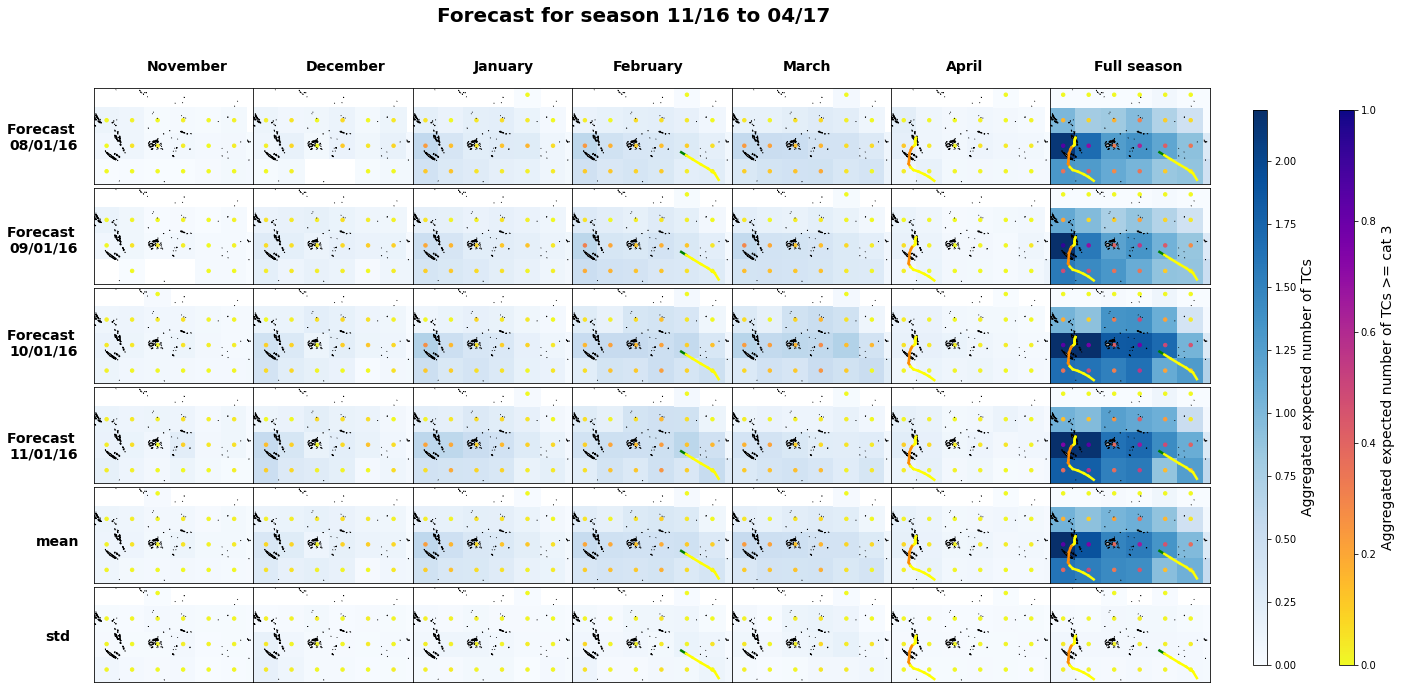
2016-2017
# TODO: no gestionar asi los output
p_season = path_f+'season_16_17/'
mean_8, mean_8_c3, std_8, std_8_c3, mean_9, \
mean_9_c3, std_9, std_9_c3, mean_10, mean_10_c3, \
std_10, std_10_c3, mean_11,mean_11_c3, std_11, \
std_11_c3, lmean, lmean_c3, lstd, lstd_c3, mean_fs, \
mean_fs_c3, mean_mean, mean_mean_c3, std_mean, \
std_mean_c3, ds4 = variables_plot_season(p_season, 2016, 5, 8)

# TODO: original 5x8 (dx dy)
#std_mean_c3, ds4 = variables_plot_season(p_season_13_14, 2013, 5, 8)
# TODO: xds_timeline??? no lo tengo
Plot_season(
    ds4, 16, 2016, 2.2, 1, mean_8, mean_8_c3,
    std_8, std_8_c3, mean_9, mean_9_c3, std_9,
    std_9_c3, mean_10, mean_10_c3, std_10, std_10_c3,
    mean_11, mean_11_c3, std_11, std_11_c3,
    lmean, lmean_c3, lstd, lstd_c3, mean_fs,
    mean_fs_c3, mean_mean, mean_mean_c3, std_mean,
    std_mean_c3, xds_timeM, 12, df,xds_timeline
);
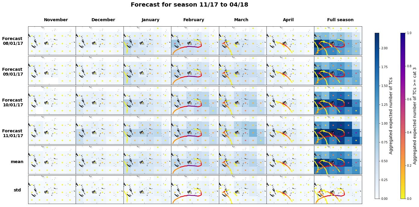
2017-2018
# TODO: no gestionar asi los output
p_season = path_f+'season_17_18/'
mean_8, mean_8_c3, std_8, std_8_c3, mean_9, \
mean_9_c3, std_9, std_9_c3, mean_10, mean_10_c3, \
std_10, std_10_c3, mean_11,mean_11_c3, std_11, \
std_11_c3, lmean, lmean_c3, lstd, lstd_c3, mean_fs, \
mean_fs_c3, mean_mean, mean_mean_c3, std_mean, \
std_mean_c3, ds4 = variables_plot_season(p_season, 2017, 5, 8)

# TODO: original 5x8 (dx dy)
#std_mean_c3, ds4 = variables_plot_season(p_season_13_14, 2013, 5, 8)
# TODO: xds_timeline??? no lo tengo
Plot_season(
    ds4, 17, 2017, 2.2, 1, mean_8, mean_8_c3,
    std_8, std_8_c3, mean_9, mean_9_c3, std_9,
    std_9_c3, mean_10, mean_10_c3, std_10, std_10_c3,
    mean_11, mean_11_c3, std_11, std_11_c3,
    lmean, lmean_c3, lstd, lstd_c3, mean_fs,
    mean_fs_c3, mean_mean, mean_mean_c3, std_mean,
    std_mean_c3, xds_timeM, 12, df,xds_timeline
);
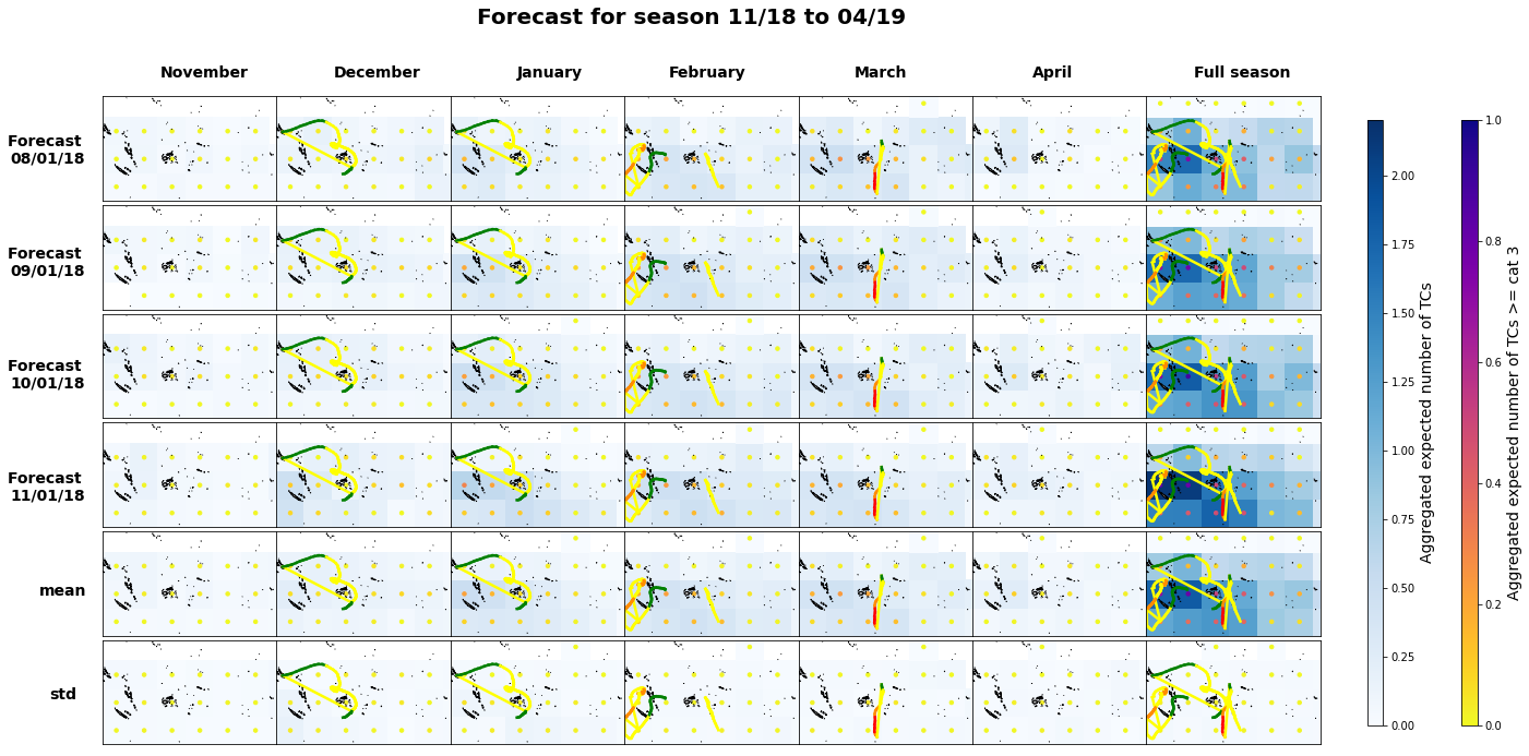
2018-2019
# TODO: no gestionar asi los output
p_season = path_f+'season_18_19/'
mean_8, mean_8_c3, std_8, std_8_c3, mean_9, \
mean_9_c3, std_9, std_9_c3, mean_10, mean_10_c3, \
std_10, std_10_c3, mean_11,mean_11_c3, std_11, \
std_11_c3, lmean, lmean_c3, lstd, lstd_c3, mean_fs, \
mean_fs_c3, mean_mean, mean_mean_c3, std_mean, \
std_mean_c3, ds4 = variables_plot_season(p_season, 2018, 5, 8)

# TODO: original 5x8 (dx dy)
#std_mean_c3, ds4 = variables_plot_season(p_season_13_14, 2013, 5, 8)
# TODO: xds_timeline??? no lo tengo
Plot_season(
    ds4, 18, 2018, 2.2, 1, mean_8, mean_8_c3,
    std_8, std_8_c3, mean_9, mean_9_c3, std_9,
    std_9_c3, mean_10, mean_10_c3, std_10, std_10_c3,
    mean_11, mean_11_c3, std_11, std_11_c3,
    lmean, lmean_c3, lstd, lstd_c3, mean_fs,
    mean_fs_c3, mean_mean, mean_mean_c3, std_mean,
    std_mean_c3, xds_timeM, 12, df,xds_timeline
);
Seasons aggregated#
seasons = [11, 12, 13, 14, 15, 16, 17, 18]

list_fs, list_fs_c3, list_mfs, list_mfs_c3, \
list_stdfs, list_stdfs_c3 = variables_plot_season_means(
    path_f, seasons, 5, 8,
)
11
12
13
14
15
16
17
18
Plot_season_means(
    ds4, df, xds_timeline, 3, 1.5, list_fs, list_fs_c3,
    list_mfs, list_mfs_c3, list_stdfs,
    list_stdfs_c3, xds_timeM, 12,
);
Forecast vs model DWTs probabilities#
#bmus from the calibration period of the methodology, from 01/1982 to 12/2019
ds_bmus = xr.Dataset(
    {
        'bmus': (('time'), xds_kma.bmus.values),
    },
    {
        'time': xds_kma.time.values,
    },
)

print(ds_bmus)
<xarray.Dataset>
Dimensions:  (time: 13879)
Coordinates:
  * time     (time) datetime64[ns] 1982-01-01 1982-01-02 ... 2019-12-31
Data variables:
    bmus     (time) int64 22 22 22 12 25 25 12 22 22 ... 18 18 18 18 23 23 23 18
s11, m11, std11, s12, m12, std12, s13, m13, \
std13, s14, m14, std14, s15, m15, std15, s16, \
m16, std16, s17, m17, std17, s18, m18, std18, \
s19, m19, std19, list_metm, list_smet = variables_dwt_forecast_plot(
    ds_bmus, 2011, path_f + 'season_',
)
Plot_forecast_dwt(
    0.3, s11, m11, std11, s12, m12, std12,
    s13, m13, std13, s14, m14, std14,
    s15, m15, std15, s16, m16, std16,
    s17, m17, std17, s18, m18, std18,
    s19, m19, std19, list_metm, list_smet,
);
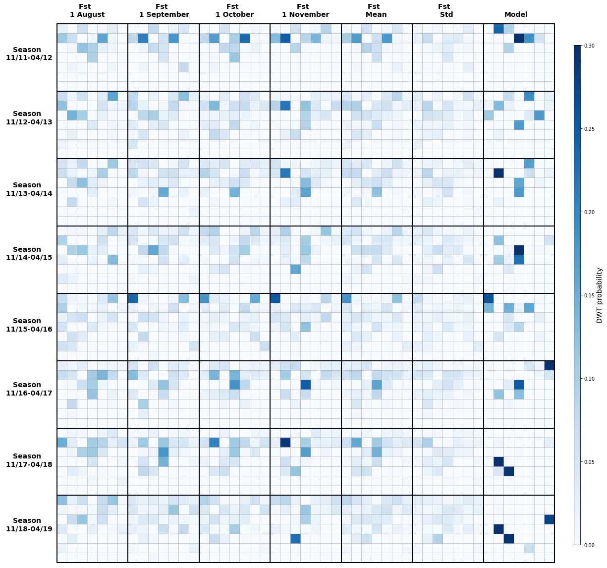
Recall:
The model performs very well when estimating the expected TC activity (number and intensity of TCs), not understimating the threat.
In some cells adjacents to the cells including TC tracks it overstimates TC activity.
Forecast performance:
Much greater uncertainty -> DWTs probability is greatly shared and therefore more extended predictand maps.
The weakness of the model are enhanced -> more extended (more overstimation in the sorroundings of the tracks) and more homogeneous maps.
When there is an unsually high TC activity (Season 15-16) the forecast understimates it in the most active cells.
Conclusion: Although the model has been proven to perform very well, the accuracy and reliability of the forecast greatly depends of the quality of the forecast data.