Statistical Downscaling Method
Contents
Statistical Downscaling Method#
DWTs chronology, seasonality and temporal variability
Relationship predictor-predictand
# common
import os
import os.path as op
import sys
import pickle as pk

# pip
import numpy as np
import pandas as pd
import xarray as xr
from sklearn.cluster import KMeans

import warnings
warnings.filterwarnings("ignore")

# DEV: bluemath
sys.path.insert(0, op.join(op.abspath(''), '..', '..', '..',  '..'))

# bluemath modules
from bluemath.seasonal_forecast_tcs.pca import PCA_seasonal_tcs_index
from bluemath.seasonal_forecast_tcs.ibtracs import load_storms_sp, dwt_tcs_count_tracks, \
ds_timeline, variables_dwt_super_plot
from bluemath.seasonal_forecast_tcs.awt import awt_mjo_ds
from bluemath.seasonal_forecast_tcs.kma import order_kma_seasonal_tcs, trmm_kma, st_bmus

from bluemath.plotting.pca import Plot_graph_variance_PCA, Plot_EOFs_seasonal_tcs_index, Plot_PCs
from bluemath.seasonal_forecast_tcs.plotting.kma import Plot_3D_kmeans, Plot_grid_kmeans
from bluemath.seasonal_forecast_tcs.plotting.dwts import custom_colorp, \
Plot_dwts_colormap, Plot_DWTs_Mean_Anom, Plot_DWTs_totalmean,Plot_Probs_WT_WT, \
Report_Sim, Chrono_dwts_tcs, Plot_DWTs_counts,Plot_DWTs_Probs, axplot_WT_Hist,Chrono_dwts_tcs
from bluemath.seasonal_forecast_tcs.plotting.tcs import Plot_DWTs_tracks
from bluemath.seasonal_forecast_tcs.plotting.calibration import Plot_calibration_period, \
Plot_calibration_period_cat3, Plot_cali_year,cluster_homogeneity

from bluemath.seasonal_forecast_tcs.awt import awt_mjo_ds,bmus_dwt_mjo
Database and site parameters#
# database
p_data = r'/media/administrador/HD2/SamoaTonga/data'
site = 'SamoaTonga'
p_site = op.join(p_data, site)

# deliverable
p_deliv = op.join(p_site, 'seasonal_forecast_tcs')

# IBTrACS database
p_ibtracs = op.join(p_data, 'IBTrACS.ALL.v04r00.nc')

# pmin, sst and mld data in the target area
p_pmin_sst_mld = op.join(p_deliv, 'df_coordinates_pmin_sst_mld.pkl')

# precipitation in target area
p_xs_trmm = op.join(p_deliv, 'xs_trmm.nc')

# index predictor values
p_sst_mld_calibration = op.join(p_deliv, 'sst_mld_calibration.nc')

#mjo and awt
p_awt = os.path.join(p_data, 'AWT_1981_2019.nc')
p_mjo = os.path.join(p_data, 'MJO_1979_2020.nc')

# output files:
p_kma = op.join(p_deliv, 'kma')

p_kma_model = op.join(p_kma, 'kma_index_okb.pkl')
p_kma_xds_index = op.join(p_kma, 'xds_kma_index_vars.nc')

if not op.isdir(p_kma):
    os.makedirs(p_kma)
# predictor parameters
lo_area = [160, 210]
la_area = [-30, 0]
Daily Weather Types (DWTs) classification#
A weather type approach is proposed.
The index predictor is first partioned into a certain number of clusters, DWTS, obtained combining three data mining techniques.
Principal Component Analysis (PCA)#
The PCA is employed to reduce the high dimensionality of the original data space and thus simplify the classification process, transforming the predictor fields into spatial and temporal modes.
# load predictor data
xs = xr.open_dataset(p_sst_mld_calibration)
xs_trmm = xr.open_dataset(p_xs_trmm)
df = pd.read_pickle(p_pmin_sst_mld)
# PCA parameters
ipca, xds_PCA = PCA_seasonal_tcs_index(xs, ['index'])

print(xds_PCA)
<xarray.Dataset>
Dimensions:        (lat: 16, lon: 26, n_components: 416, n_features: 416, n_points: 416, time: 13879)
Coordinates:
  * lon            (lon) float64 160.2 162.2 164.2 166.2 ... 206.2 208.2 210.2
  * lat            (lat) float64 -0.25 -2.25 -4.25 ... -26.25 -28.25 -30.25
Dimensions without coordinates: n_components, n_features, n_points, time
Data variables:
    PCs            (time, n_components) float64 6.632 -0.6629 ... -0.6441 0.2296
    EOFs           (n_components, n_features) float64 -0.0165 ... -0.04901
    variance       (n_components) float64 131.1 25.34 15.42 ... 0.1458 0.1413
    pred_mean      (n_features) float64 0.5407 0.5346 0.521 ... 0.1504 0.09442
    pred_std       (n_features) float64 0.2985 0.3022 0.3003 ... 0.189 0.1484
    pred_time      (time) datetime64[ns] 1982-01-01 1982-01-02 ... 2019-12-31
    pred_data_pos  (n_points) bool True True True True ... True True True True
Attributes:
    method:     gradient + estela + sea mask
    pred_name:  ['index']
xds_PCA.to_netcdf(os.path.join(p_deliv, 'xds_pca.nc'))
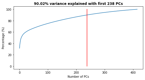
PCA projects the original data on a new space searching for the maximum variance of the sample data.
The first 237 PCs are captured, which explain the 90 % of the variability as shown:
variance_PCA = Plot_graph_variance_PCA(xds_PCA)
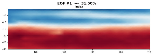
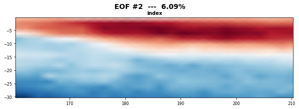
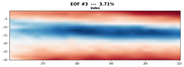
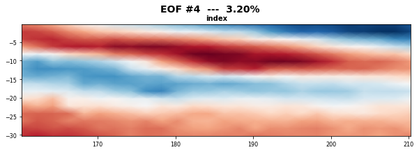
The eigenvectors (the empirical orthogonal functions, EOFs) of the data covariance matrix define the vectors of the new space.
They represent the spatial variability.
Plot_EOFs_seasonal_tcs_index(xds_PCA, 4);
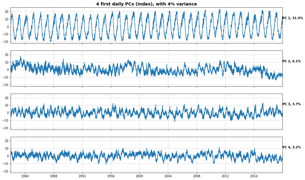
The PCs represent the temporal variability.
fig_PCA = Plot_PCs(xds_PCA, 4)
K-means clustering#
Daily synoptic patterns of the index predictor are obtained using the K-means clustering algorithm. It divides the data space into 49 clusters, a number that which must be a compromise between an easy handle characterization of the synoptic patterns and the best reproduction of the variability in the data space. Previous works with similar anlaysis confirmed that the selection of this number is adequate (Rueda et al. 2017).
Each cluster is defined by a prototype and formed by the data for which the prototype is the nearest.
Finally the best match unit (bmus) of daily clusters are reordered into a lattice following a geometric criteria, so that similar clusters are placed next to each other for a more intuitive visualization.
# PCA data
variance = xds_PCA.variance.values[:]
EOFs = xds_PCA.EOFs.values[:]
PCs = xds_PCA.PCs.values[:]

var_anom_std = xds_PCA.pred_std.values[:]
var_anom_mean = xds_PCA.pred_mean.values[:]
time = xds_PCA.time.values[:]

variance = xds_PCA.variance.values
percent = variance / np.sum(variance)*100
percent_ac = np.cumsum(percent)
n_comp_95 = np.where(percent_ac >= 95)[0][0]
n_comp_90 = np.where(percent_ac >= 90)[0][0]

# plot
n_comp = n_comp_90 # 90% variance explained with 238 PCs

nterm = n_comp_90 + 1
PCsub = PCs[:, :nterm]
EOFsub = EOFs[:nterm, :]

# normalization
data = PCsub
data_std = np.std(data, axis=0)
data_mean = np.mean(data, axis=0)
# normalize but keep PCs weigth
data_norm = np.ones(data.shape)*np.nan
for i in range(PCsub.shape[1]):
    data_norm[:,i] = np.divide(data[:,i] - data_mean[i], data_std[0])

# KMeans classification
num_clusters = 49
kma = KMeans(n_clusters=num_clusters, n_init=1000).fit(data_norm)
kma

# store kma model
with open(p_kma_model, "wb") as f:
    pk.dump(kma, f)

# # load kma model
# with open(p_kma_model, "rb") as f:
#     kma = pk.load(f)


#a measure of the error of the algorithm
kma.inertia_
19797.971871059028
xds_kma_ord, xds_kma = order_kma_seasonal_tcs(kma, xds_PCA, xs)

# store index kma
xds_kma.to_netcdf(p_kma_xds_index)
Kma order obtained:  [25 11 39 17  7  4 36 18 43 14 28 21  0  2 19 34 26 40 46 12 37  6 31 24
 29  3 41 10 23 22 33 47 27 13 30 16  9  1 38 44 15 48  8 35 42 32 45  5
 20]
xds_kma_ord.to_netcdf(p_kma+'/xds_kma_ord.nc')
xds_kma_sel = trmm_kma(xds_kma, xs_trmm)
xds_kma_sel.to_netcdf(p_kma+'/xds_kma_sel.nc')
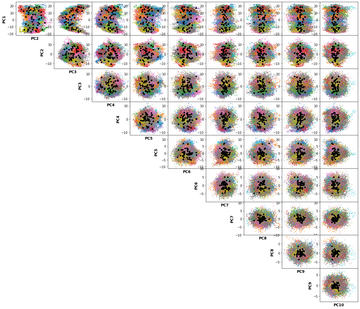
The resulting classification can be seen in the PCs space of the predictor index data. The obtained centroids (black dots), span the wide variability of the data.
# CHECKUP PLOT 3D
#%matplotlib inline
fig = Plot_3D_kmeans(
    xds_kma_ord, xds_kma_ord.bmus.values,
    xds_kma_ord.cenEOFs.values,
    figsize = (12, 10),
);
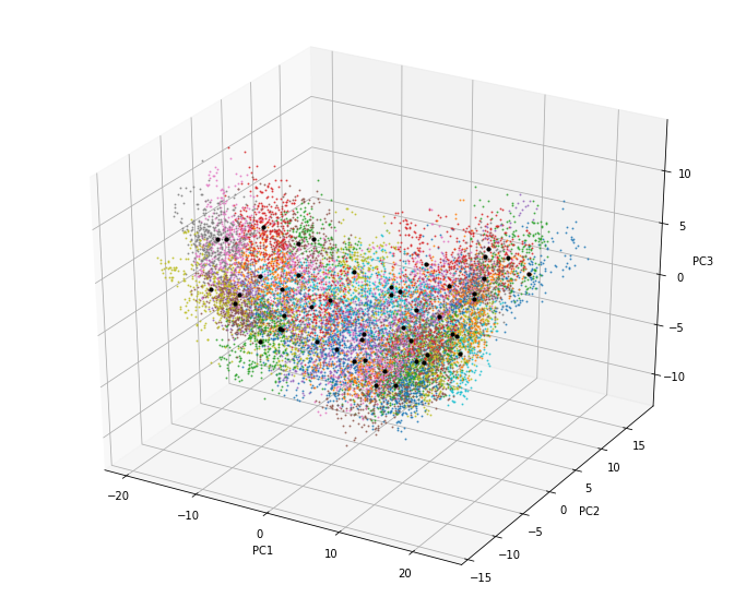
fig = Plot_grid_kmeans(
    xds_kma_ord, xds_kma_ord.bmus.values,
    xds_kma_ord.cenEOFs.values,
    9, ibmus = range(49),
    figsize = (20, 18),
);
DWTs plotting#
# load TCs
xds_ibtracs, xds_SP = load_storms_sp(p_ibtracs)
All basins storms:  13549
SP basin storms:    1130
st_bmus, st_lons, st_lats, st_categ = st_bmus(xds_SP, xds_kma)
# custom colorbar for index
color_ls = [
    'white','cyan','cornflowerblue',
    'darkseagreen','olivedrab','gold',
    'darkorange','orangered','red',
    'deeppink','violet','darkorchid',
    'purple','midnightblue',
]
custom_cmap = custom_colorp(color_ls)
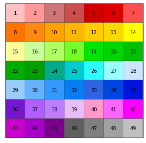
DWTs lattice and corresponding colors:
Plot_dwts_colormap(xds_kma.n_clusters.size);
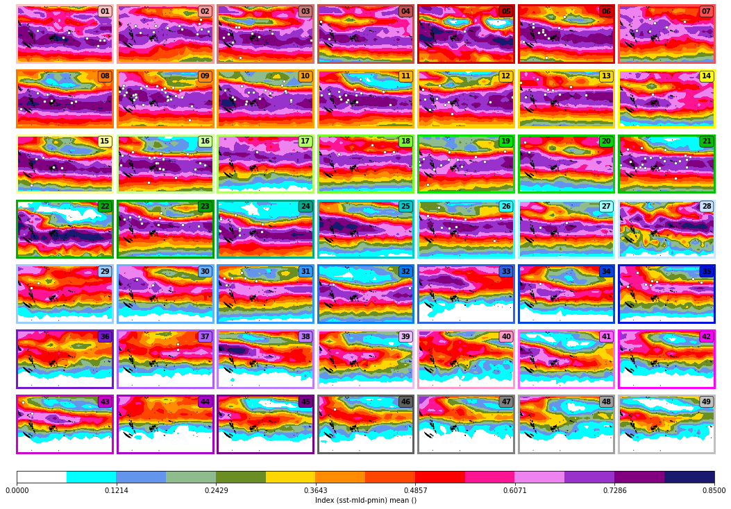
The resulting clustering of the index predictor, each cell is the mean of all the patterns of the corresponding cluster:
Plot_DWTs_Mean_Anom(
    xds_kma, xs, ['index'],
    minis = [0], maxis = [.85],
    levels = [len(color_ls)],
    kind='mean',
    cmap = [custom_cmap],
    genesis ='on',
    st_bmus = st_bmus,
    st_lons = st_lons,
    st_lats = st_lats,
    markercol = 'white',
    markeredge = 'k',
    figsize = (18, 12),
);
index: min(0.0) max(1.0)
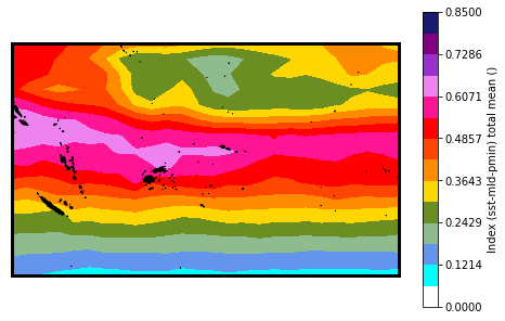
DWTs (index) total mean:
Plot_DWTs_totalmean(
    xs, ['index'],
    minis = [0], maxis = [.85],
    levels = [len(color_ls)],
    cmap = [custom_cmap],
);
index: min(0.1) max(0.7)
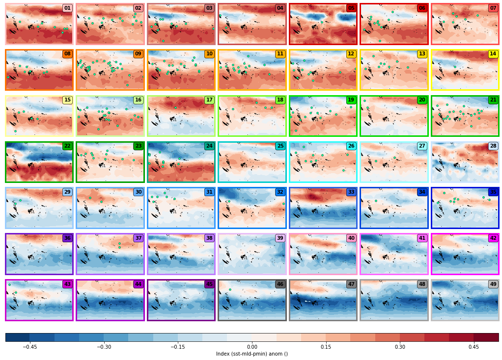
DWTs (index) Anomalies:
Plot_DWTs_Mean_Anom(
    xds_kma, xs, ['index'],
    minis = [-.5], maxis = [.5],
    levels = [20],
    kind = 'anom',
    cmap = ['RdBu_r'],
    genesis = 'on',
    st_bmus = st_bmus,
    st_lons = st_lons,
    st_lats = st_lats,
    markercol = 'mediumspringgreen',
    markeredge = 'k',
    figsize = (18, 12),
);
Cluster homegeinity#
The DWTs are different to each other, showing the high variability of the data space. The clusters are also very homogenous inside. This confirms 49 as a good choice, which additionally is a manageable number.
n=10
fig = cluster_homogeneity(xds_kma,n,color_ls,custom_cmap)

DWTs plotting with predictand variables#
# custom colorbar for sst
color_ls = [
"dimgrey", "darkgrey","lightgrey","darkorchid","purple",
"midnightblue","blue","royalblue","cyan","turquoise",
"green","olive","darkkhaki","gold","darkorange",
"orangered", "red","deeppink","violet","lightpink",
]
custom_cmap = custom_colorp(color_ls)
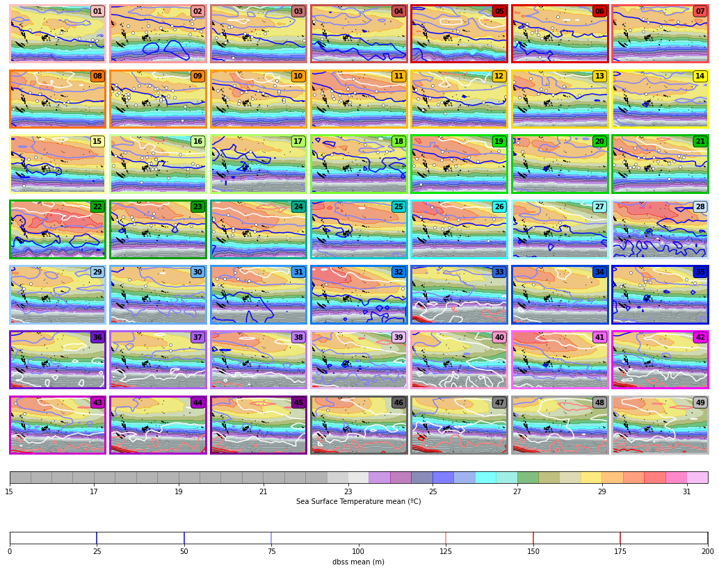
Plot_DWTs_Mean_Anom(
xds_kma, xs, ['sst', 'dbss'],
minis = [22, 0],
maxis = [32, 200],
levels = [(32-22)/0.5, 8],
kind = 'mean',
cmap=[custom_cmap, 'seismic'],
genesis = 'on',
st_bmus = st_bmus,
st_lons = st_lons,
st_lats = st_lats,
markercol = 'white',
markeredge = 'k',
figsize = (18, 12),
);
sst: min(14.899999618530273)  max(33.0)
dbss: min(7.5)  max(330.0)
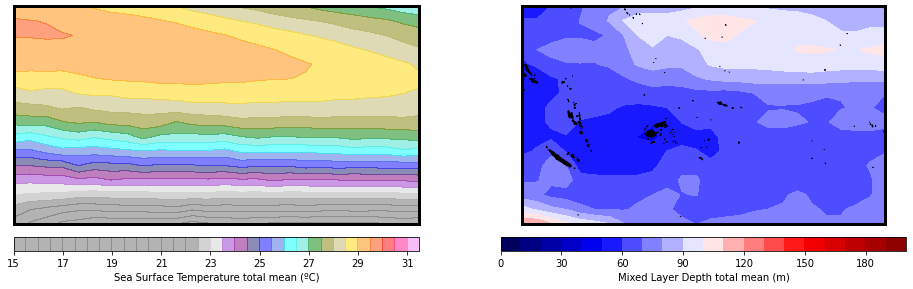
DWTs - SST and MLD total mean:
Plot_DWTs_totalmean(
    xs, ['sst','dbss'],
    minis = [22, 0],
    maxis = [32, 200],
    levels = [(32-22)/0.5,20],
    cmap = [custom_cmap, 'seismic'],
);
sst: min(20.299999237060547)  max(29.5)
dbss: min(46.20000076293945)  max(120.0)
DWTs - SST and MLD Anomalies:
Plot_DWTs_Mean_Anom(
    xds_kma, xs, ['sst', 'dbss'],
    minis = [-4, -60],
    maxis = [4, 60],
    levels = [20, 6],
    kind = 'anom',
    cmap = ['coolwarm', 'seismic'],
    genesis = 'on',
    st_bmus = st_bmus,
    st_lons = st_lons,
    st_lats = st_lats,
    markercol = 'mediumspringgreen',
    markeredge = 'k',
    figsize = (18, 12),
);
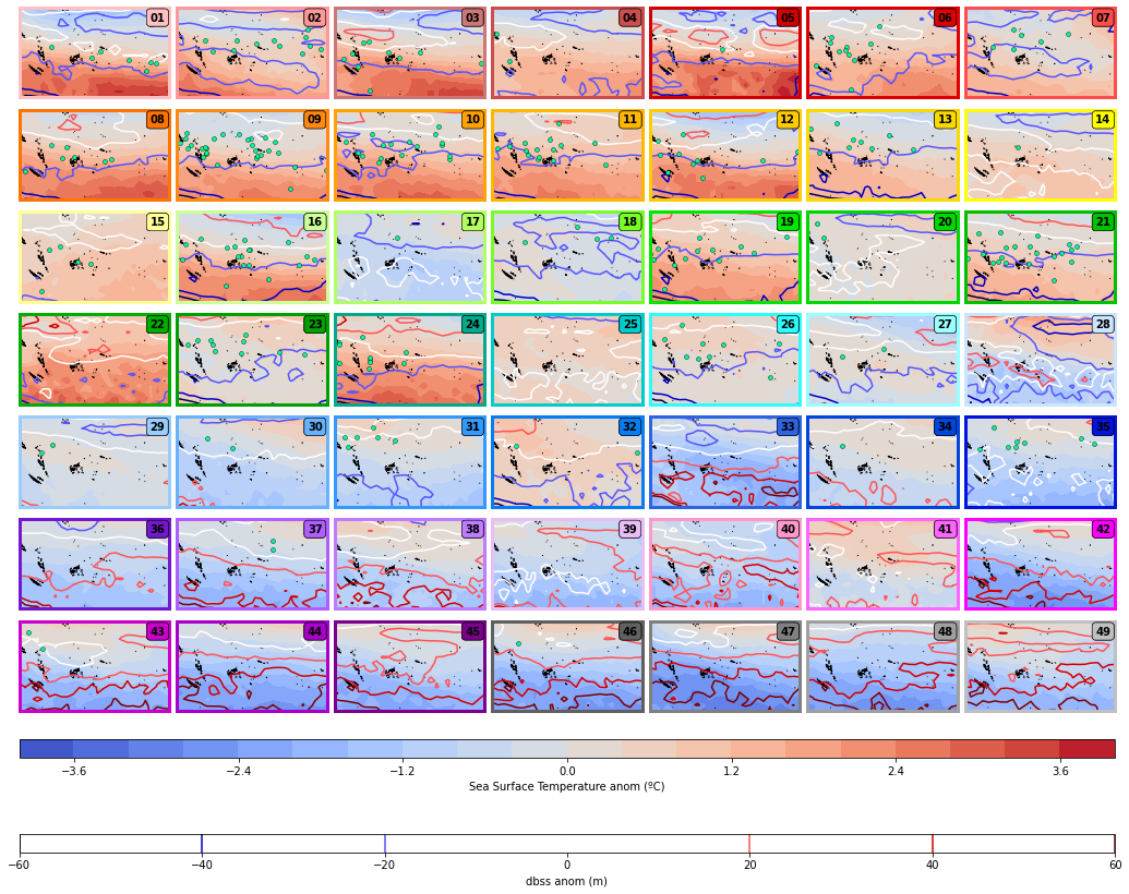
Clear patterns can be extracted from these figures related to TCs genesis. Most of it takes place under the following conditions:
SST interval from 28ºC to 30ºC (specially 28.5 to 29.5 ºC) that correspond to positive or zero SST anomalies.
MLD values equal or smaller to 75 m that correspond to negative anomalies.
DWTs seasonality, annual variability and chronology#
Several plots are shown to better analyse the distribution of DWTs, their transition, persistence and conditioning to TCs occurrence and to AWT.
awt, mjo, awt0 = awt_mjo_ds(p_mjo, p_awt)
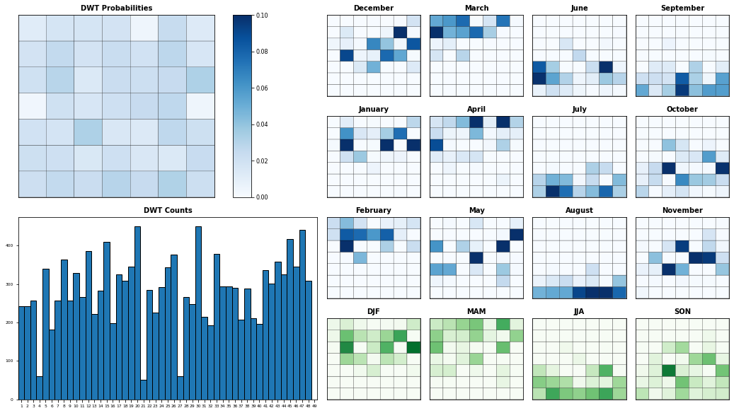
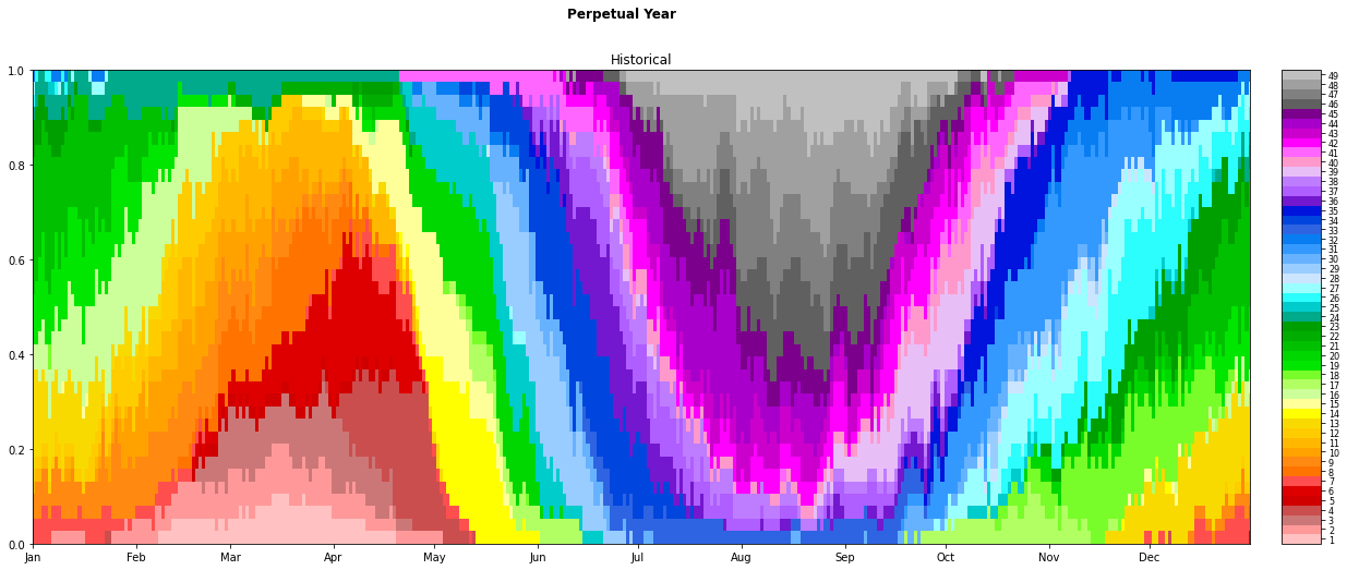
Seasonality:
bmus_DWT, bmus_time, awt0_sel_bmus, bmus_AWT, bmus_MJO = bmus_dwt_mjo(mjo, awt, awt0, xds_kma)
Plot_DWTs_Probs(bmus_DWT, bmus_time, 49, figsize = (18, 10));
p_count_tcs_8 = os.path.join(p_deliv, 'xds_count_tcs_8.nc')
p_count_tcs_8_964 = os.path.join(p_deliv, 'xds_count_tcs_8_964.nc')
p_count_tcs_8_979 = os.path.join(p_deliv, 'xds_count_tcs_8_979.nc')
# all categories
xs_dwt_counts = dwt_tcs_count_tracks(
    xds_kma, df,
    dx = 8, dy = 8,
    lo0 = lo_area[0], lo1 = lo_area[1],
    la0 = la_area[0], la1 = la_area[1],
)
xs_dwt_counts.to_netcdf(p_count_tcs_8)

# category 3
xs_dwt_counts_964 = dwt_tcs_count_tracks(
    xds_kma, df,
    dx = 8, dy = 8,
    categ = 965,
    lo0 = lo_area[0], lo1 = lo_area[1],
    la0 = la_area[0], la1 = la_area[1],
)
xs_dwt_counts_964.to_netcdf(p_count_tcs_8_964)

# category 2
xs_dwt_counts_979 = dwt_tcs_count_tracks(
    xds_kma, df,
    dx = 8, dy = 8,
    categ = 979,
    lo0 = lo_area[0], lo1 = lo_area[1],
    la0 = la_area[0], la1 = la_area[1],
)
xs_dwt_counts_979.to_netcdf(p_count_tcs_8_979)
#load counts
xs_dwt_counts = xr.open_dataset(p_count_tcs_8)
xs_dwt_counts_964 = xr.open_dataset(p_count_tcs_8_964)
xs_dwt_counts_979 = xr.open_dataset(p_count_tcs_8_979)
xds_timeline = ds_timeline(df, xs_dwt_counts, xs_dwt_counts_964, xds_kma)
mask_bmus_YD, mask_tcs_YD = variables_dwt_super_plot(xds_kma, xds_timeline)
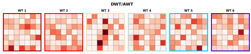
AWT transferred to the DWTs:
#  TODO: solucionar archivo awt_mjo_ds y descomentar

n_clusters_AWT = 6
n_clusters_DWT = 49
n_clusters_MJO = 8

Plot_Probs_WT_WT(
    bmus_AWT, bmus_DWT,
    n_clusters_AWT, n_clusters_DWT,
    ttl = 'DWT/AWT',
    wt_colors = True,
    figsize = (15, 3),
);
Chronology:
Report_Sim(xds_kma, py_month_ini=1);
Chronology during all the calibration period, with the AWT on the left and the TC days included as black dots:
# TODO: solucionar archivo awt_mjo_ds y descomentar

Chrono_dwts_tcs(xds_kma, mask_bmus_YD, mask_tcs_YD, awt0_sel_bmus);
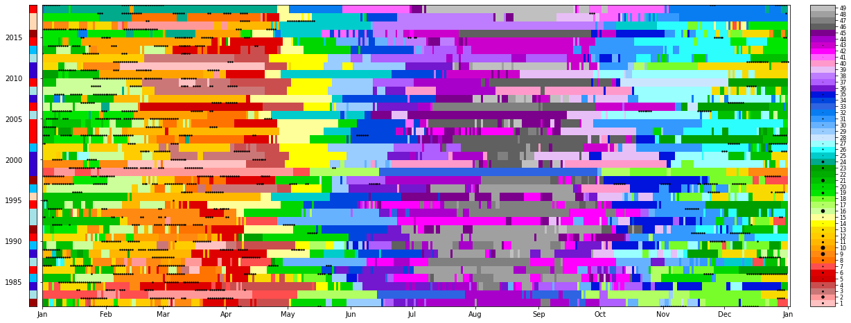
During the TC season months (November, December, January, February, March and April) the DWTs proability is focused on the upper half of the upper part of the lattice, where most of the TC genesis is also concentrated. In the most intense months (January, February and March) DWTs with the highest number of TCs genesis points are especially likely. On the contrary, in the rest of the months, the probability is shared amongst the DWTs of the lower half of the lattice, where there is very few or null TC genesis activity.
Intra annual variability:
Months out of the TCs season: purple, pink, gray and blue -> DWTs from 29 to 49 -> low or null TCs genesis activity.
Months out of the TCs season: green, orange, red, yellow -> DWTs from 1 to 28 -> high TCs genesis acitvity.
Interanual varibility:
El Niño: not much variability, high TC activity (DWTs like 6 or 18 are very probable), 1997 is the year when the season starts earlier (October) and ends later (June)
Other factors influences such as long-terms trends, maybe associated to SST warming during this time period.
Relationship predictor-predictand#
DWTs storm frequency and track counting#
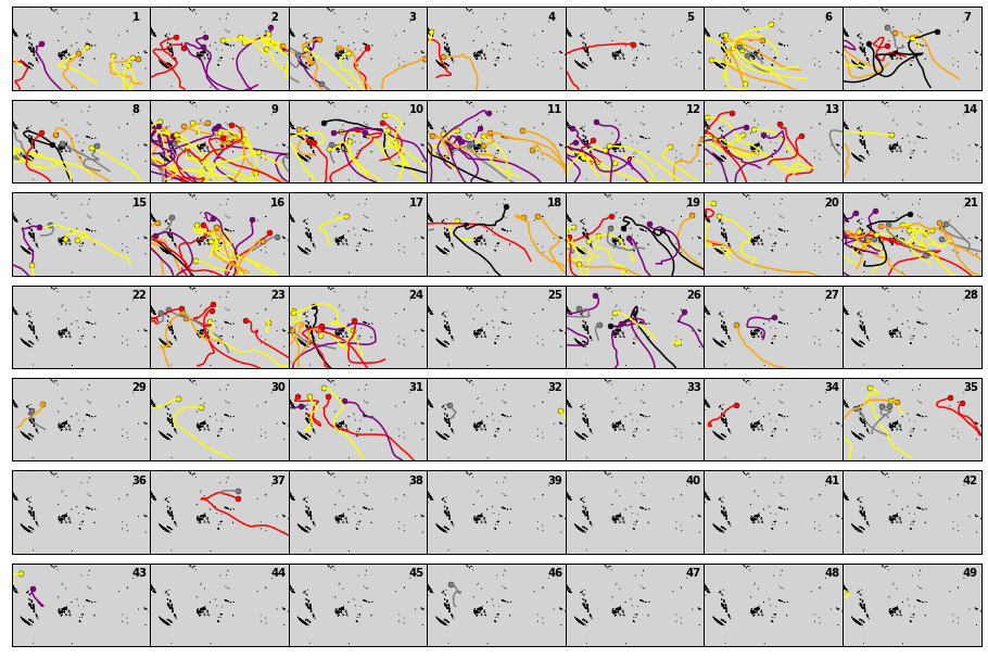
DWTs - TCs tracks according to genesis
Plot_DWTs_tracks(
    xds_kma, xs,
    st_bmus, st_lons, st_lats, st_categ,
    mode = 'genesis',
    cocean = 'lightgray',
);
DWTs - TCs tracks segments
fig = Plot_DWTs_tracks(
    xds_kma, xs,
    st_bmus, st_lons, st_lats, st_categ,
    mode = 'segments',
    cocean = 'lightgray',
);
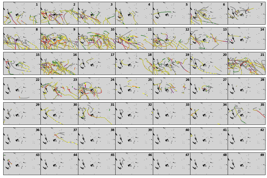
Considering only the genesis point as the transfer criteria to the DWTs make us miss some important information since the TCs tracks develop along many days, during which the DWT can change.
The predictor area is discretized in squared 8º cells to compute the storm frequency per DWT.
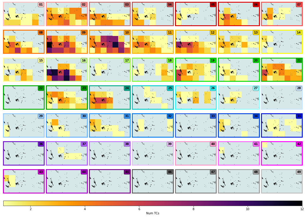
Absolute number of TCs per DWT:
Plot_DWTs_counts(xs_dwt_counts, mode = 'counts_tcs');
counts_tcs: min(1.0) max(12.0)
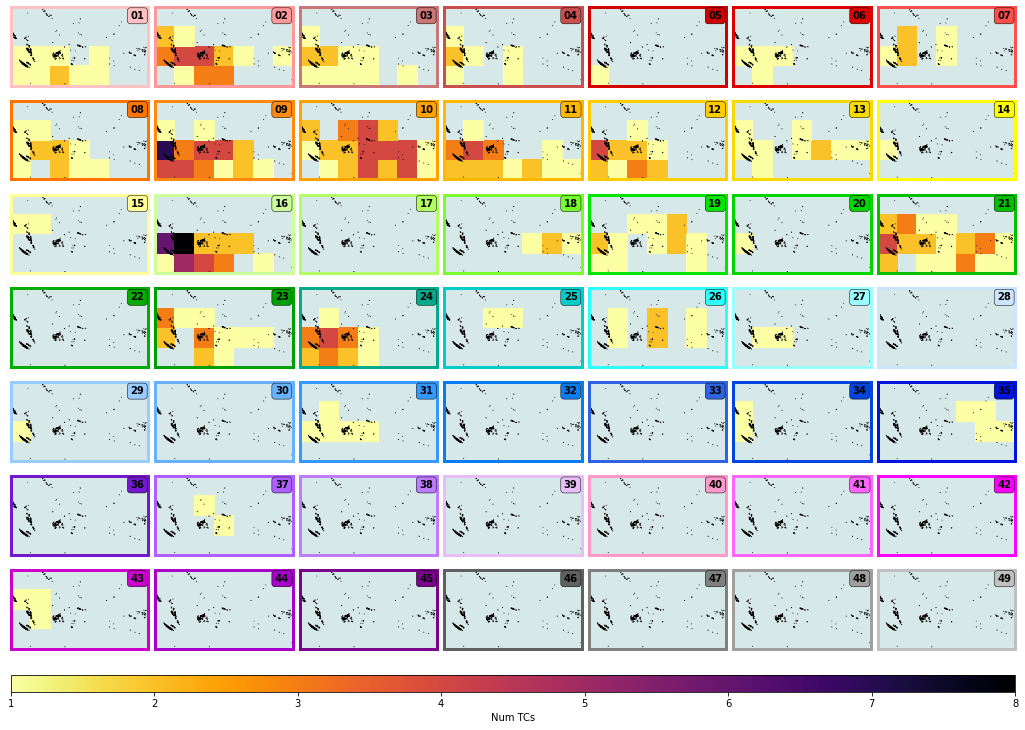
Absolute number of TCs reaching category 2 or greater per DWT:
Plot_DWTs_counts(xs_dwt_counts_979, mode = 'counts_tcs');
counts_tcs: min(1.0) max(8.0)
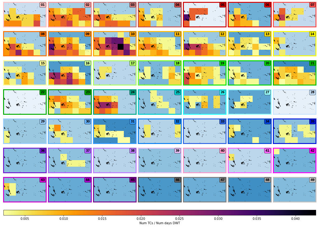
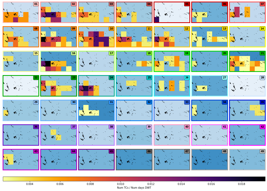
Number of TCs per day conditioned to each DWT, with DWT probability as background color:
Plot_DWTs_counts(xs_dwt_counts, mode = 'tcs_dwts');
tcs_dwts: min(0.0022172949002217295) max(0.04263565891472868)
Number of TCs reaching category 2 or greater per day conditioned to each DWT, with DWT probability as background color:
Plot_DWTs_counts(xs_dwt_counts_979, mode = 'tcs_dwts');
tcs_dwts: min(0.0022172949002217295) max(0.019559902200488997)
Calibration time period predictand plotting #
Recall:
Generation of the index predictor.
Clustering of the index predictor in 49 synoptic patterns named DWTs.
Calculation of the number of TCs per day conditioned to each DWT in 8x8º cells in the target area.
Each day of the calibration period has therefore its expected number of TCs map.
xds_timeline = ds_timeline(df, xs_dwt_counts, xs_dwt_counts_964, xds_kma)
This mean expected daily number of TCs in 8x8º cells is aggregated in monthly basis for an easy management and visualization.
# resample months
xds_timeM0 = xds_timeline.resample(time='MS', skipna=True).sum()
del xds_timeM0['bmus']

xds_timeM = xds_timeM0.where(xds_timeM0.probs_tcs > 0, np.nan)
xds_timeM.to_netcdf(p_deliv+'/xds_timeM.nc')
print(xds_timeM)
<xarray.Dataset>
Dimensions:         (lat: 5, lon: 8, time: 456)
Coordinates:
  * time            (time) datetime64[ns] 1982-01-01 1982-02-01 ... 2019-12-01
  * lat             (lat) int64 -30 -22 -14 -6 2
  * lon             (lon) int64 160 168 176 184 192 200 208 216
Data variables:
    mask_tcs        (time, lat, lon) float64 8.0 8.0 8.0 8.0 ... nan nan nan nan
    counts_tcs      (time, lat, lon) float64 98.0 69.0 85.0 70.0 ... nan nan nan
    counts_tcs_964  (time, lat, lon) float64 23.0 23.0 19.0 18.0 ... nan nan nan
    probs_tcs       (time, lat, lon) float64 0.3262 0.2307 0.2931 ... nan nan
    probs_tcs_964   (time, lat, lon) float64 0.07657 0.0737 0.06591 ... nan nan
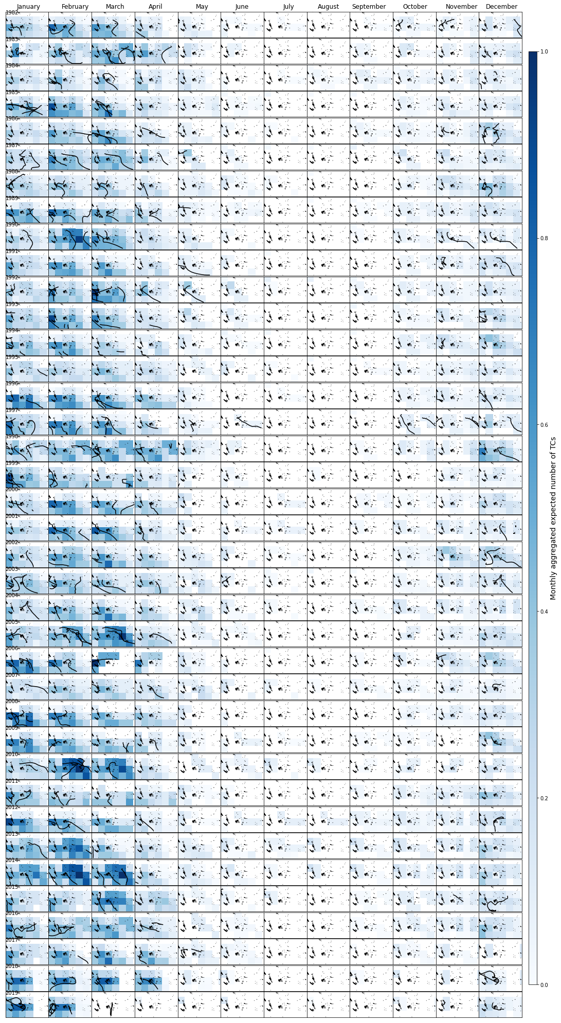
Expected mean number of TCs in 8x8º cells in the target area for the calibration time period (1982-2019), including the historical TC tracks:
Plot_calibration_period(xds_timeM, xds_timeline, df, 1, lo_area, la_area);
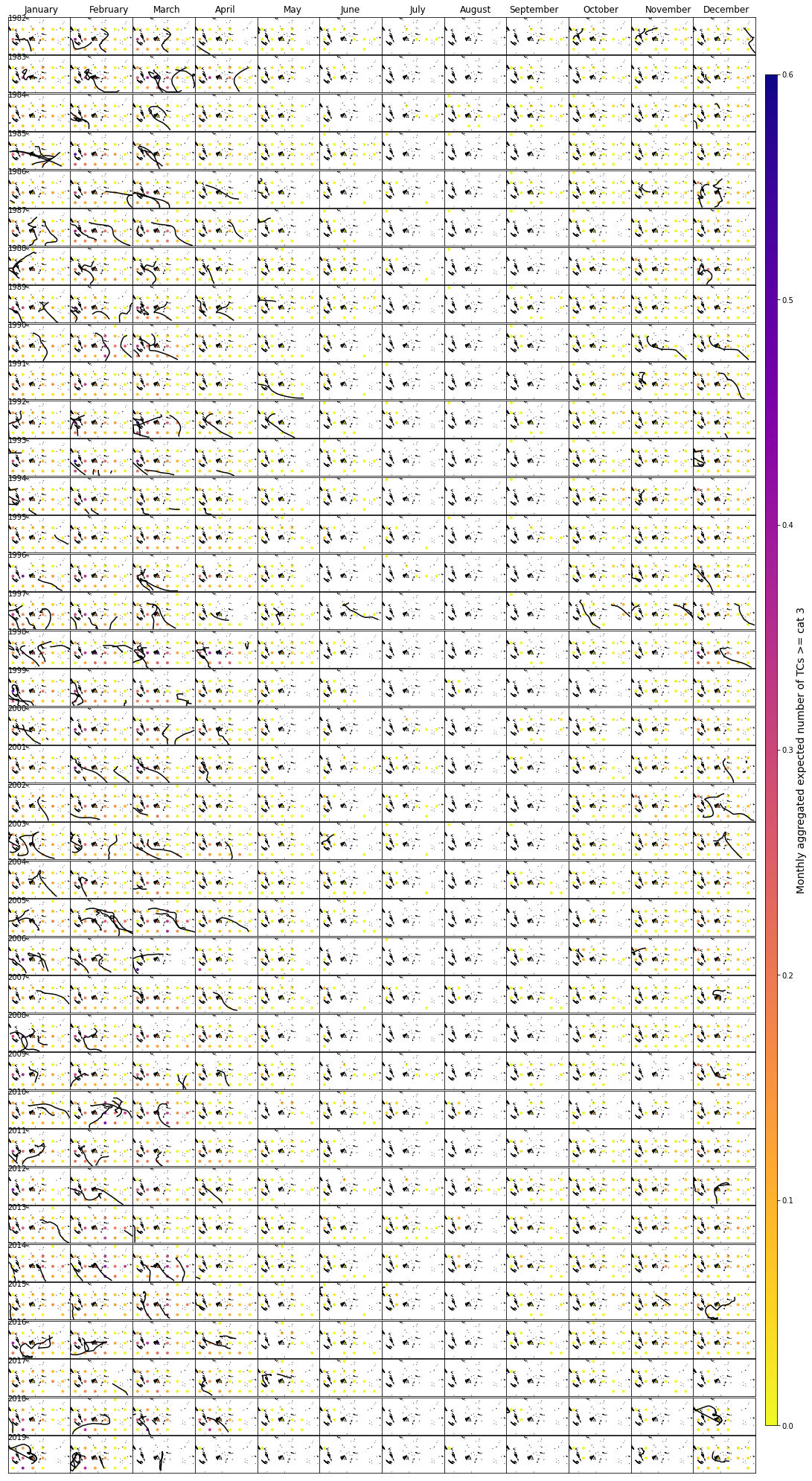
Expected number of TCs reaching category 3 or greater in 8x8º cells in the target area for the calibration time period (1982-2019), including the historical TC tracks:
Plot_calibration_period_cat3(xds_timeM, xds_timeline, df, 0.6, 8, lo_area, la_area);
Expected number of TCs in 8x8º cells in the target area for year 2015 (El Niño) of the calibration time period (1982-2019) including the historical TC tracks coloured according to their category:
Plot_cali_year(2015, xds_timeline, xds_timeM, df, 35, lo_area, la_area, figsize = (18, 15));
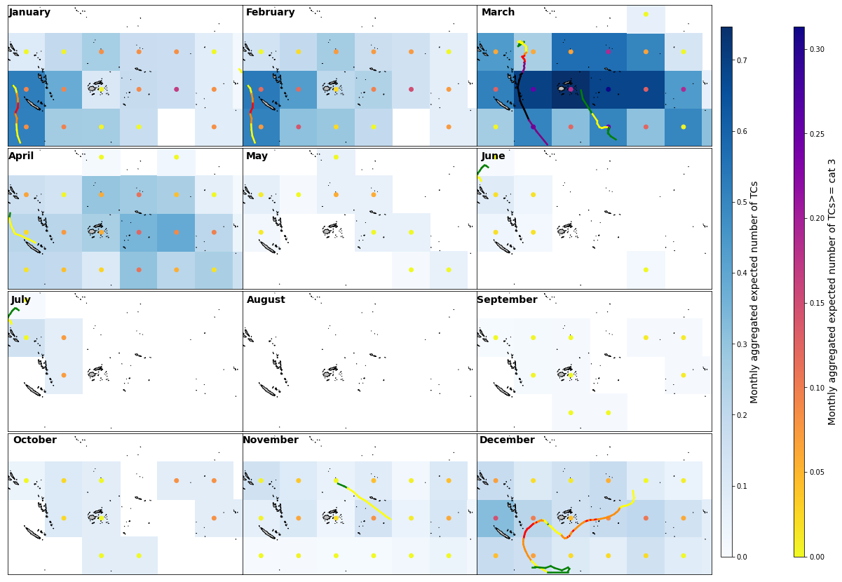
The model generally performs very well since it effectively and accuretly estimates the TC activity (quantity and intensity of TCs).
In some zones (depending on the month) the model overstimates the number of TCs since rather than predicting the exact path followed by the TC track it predicts the track and its area of infuence (surroundings).
When a TC is very intense or very close in dates to the previous or following month it leaves its footprint (like Pam from 07/03/2015 in February).