Model Validation
Contents
Model Validation#
# common
import os
import os.path as op
import sys
import pickle as pk
#import pickle5 as pk5

# pip
import numpy as np
import pandas as pd
import xarray as xr

import warnings
warnings.filterwarnings("ignore")

# DEV: bluemath
sys.path.insert(0, op.join(op.abspath(''), '..', '..', '..', '..'))

# bluemath modules
from bluemath.seasonal_forecast_tcs.validation import change_sst_resolution, \
ds_index_over_time, ds_monthly_probabilities, PCA_k_means_val

from bluemath.seasonal_forecast_tcs.pca import PCA_k_means

from bluemath.seasonal_forecast_tcs.plotting.validation import Plot_bmus_chronology, Plot_scatter_kmeans, \
Plot_bmus_comparison_validation_calibration, Plot_validation_year, Plot_validation_full_season
Database and site parameters#
# mld and sst
p_mld = '/media/administrador/HD1/DATABASES/SeasonalForecast_TCs/CFS/ocnmld'
p_sst = '/media/administrador/HD1/DATABASES/SeasonalForecast_TCs/SST'
p_mld_1982 = op.join(p_mld+'/ocnmld.day.mean.1982.nc')

# database

p_data = r'/media/administrador/HD2/SamoaTonga/data'
site = 'SamoaTonga'
p_site = op.join(p_data, site)

# deliverable
p_deliv = op.join(p_site, 'seasonal_forecast_tcs')

# IBTrACS database
p_ibtracs = op.join(p_data, 'IBTrACS.ALL.v04r00.nc')

#KMA model
p_kma = op.join(p_deliv, 'kma')
p_kma_model = op.join(p_deliv, 'kma', 'kma_index_okb.pkl')

# index predictor values
p_sst_mld_slp_calibration = op.join(p_deliv, 'sst_mld_slp_calibration.nc')

# precipitation in target area
p_xs_trmm = op.join(p_deliv, 'xs_trmm.nc')
xs = xr.open_dataset(p_sst_mld_slp_calibration)

xds_kma =  xr.open_dataset(p_kma+'/xds_kma_index_vars.nc')
xds_kma_sel =  xr.open_dataset(p_kma+'/xds_kma_sel.nc')
xds_kma_ord = xr.open_dataset(p_kma+'/xds_kma_ord.nc')

xds_count_tcs_8 = xr.open_dataset(p_deliv+'/xds_count_tcs_8.nc')
xds_count_tcs_8_964 = xr.open_dataset(p_deliv+'/xds_count_tcs_8_964.nc')
xds_count_tcs_8_979 = xr.open_dataset(p_deliv+'/xds_count_tcs_8_979.nc')

xds_PCA = xr.open_dataset(p_deliv+'/xds_pca.nc')
xds_timeM = xr.open_dataset(p_deliv+'/xds_timeM.nc')

df_2021 = pd.read_pickle(p_deliv+'/df_coordinates_pmin_sst_mld_2021.pkl')
df_2019 = pd.read_pickle(p_deliv+'/df_coordinates_pmin_sst_mld.pkl')
# predictor parameters
lo_area = [160, 210]
la_area = [-30, 0]

#lo_SP, la_SP = [130, 250], [-60, 0]
lop1 = 160.25
lop2 = 211
lap1 = -0.25
lap2 = -32
delta = 2
After analizing the tailor-made predictor along the hindcast data for the calibration period (1982-2019), the performace of the model will be validated for year 2020, which has not been included in the predictor calibration process.
Steps:
1. Download and preprocess (file conversion and resolution interpolation) SST and MLD data for the validation time period.
2. Generation of the index predictor based on the index function obtained at the calibration period.
3. The fitted Principal Component Analysis for the calibration is used to predict the index principal components in that same temporal-spatial space.
4. The predicted PCs are assigned to the best match unit group from the fitted K-means clustering -> based on the index predictor a DWT is assigned to each day.
5. From the DWT the expected daily mean number of TCs in 8x8º cells map in the target area is known.
Index predictor and DWTs#
Download and preprocess (file conversion and resolution interpolation) SST and MLD data for the validation time period.
# load mld and sst data for preprocessing
mld_ref = xr.open_dataset(p_mld_1982)

year_val = 2020
p_mld_val  = op.join(p_mld+'/ocnmld.day.mean.{0}.nc'.format(year_val))
p_sst_val  = op.join(p_sst+ '/sst.day.mean.{0}.nc'.format(year_val))

sst_val = xr.open_dataset(p_sst_val)
mld_val = xr.open_dataset(p_mld_val)
sst_val_0505 = change_sst_resolution(mld_ref, sst_val)
sst_val_0505.to_netcdf(p_deliv+'/sst.day.mean.{0}.0505.nc'.format(year_val))
Generation of the index predictor based on the index function obtained at the calibration period.
# generate index for validation period
xs_val = ds_index_over_time(df_2019, sst_val_0505, mld_val, lop1, lop2, lap1, lap2, delta)
xs_val
<xarray.Dataset>
Dimensions:  (lat: 16, lon: 26, time: 366)
Coordinates:
  * time     (time) datetime64[ns] 2020-01-01 2020-01-02 ... 2020-12-31
  * lat      (lat) float64 -0.25 -2.25 -4.25 -6.25 ... -26.25 -28.25 -30.25
  * lon      (lon) float64 160.2 162.2 164.2 166.2 ... 204.2 206.2 208.2 210.2
Data variables:
    index    (time, lat, lon) float64 0.0 0.05833 0.0 0.0 ... 0.0 0.0 0.0 0.0
    sst      (time, lat, lon) float32 30.49 29.95 29.35 ... 23.67 23.79 24.02
    dbss     (time, lat, lon) float32 98.42 106.0 109.8 ... 13.58 13.92 12.21
mask (lat, lon) float64 0.0 0.0 0.0 0.0 0.0 0.0 ... 0.0 0.0 0.0 0.0 0.0- lat: 16
- lon: 26
- time: 366
- time(time)datetime64[ns]2020-01-01 ... 2020-12-31
array(['2020-01-01T00:00:00.000000000', '2020-01-02T00:00:00.000000000', '2020-01-03T00:00:00.000000000', ..., '2020-12-29T00:00:00.000000000', '2020-12-30T00:00:00.000000000', '2020-12-31T00:00:00.000000000'], dtype='datetime64[ns]') - lat(lat)float64-0.25 -2.25 -4.25 ... -28.25 -30.25
array([ -0.25, -2.25, -4.25, -6.25, -8.25, -10.25, -12.25, -14.25, -16.25, -18.25, -20.25, -22.25, -24.25, -26.25, -28.25, -30.25]) - lon(lon)float64160.2 162.2 164.2 ... 208.2 210.2
array([160.25, 162.25, 164.25, 166.25, 168.25, 170.25, 172.25, 174.25, 176.25,
       178.25, 180.25, 182.25, 184.25, 186.25, 188.25, 190.25, 192.25, 194.25,
       196.25, 198.25, 200.25, 202.25, 204.25, 206.25, 208.25, 210.25])
- index(time, lat, lon)float640.0 0.05833 0.0 0.0 ... 0.0 0.0 0.0
- varname :
- Index (sst-mld-pmin)
- units :
array([[[0. , 0.05833333, 0. , ..., 0. , 0.53333333, 0. ], [0. , 0.14166667, 0.04166667, ..., 0.575 , 0.53333333, 0.15833333], [0.2 , 0. , 0.04166667, ..., 0. , 0. , 0.53333333], ..., [0.53333333, 0.53333333, 0.575 , ..., 0.16666667, 0.36666667, 0.36666667], [0.53333333, 0.28333333, 0.61666667, ..., 0.24166667, 0. , 0.01666667], [0.36666667, 0.40833333, 0.40833333, ..., 0.24166667, 0. , 0. ]], [[0. , 0. , 0. , ..., 0. , 0.15833333, 0.65833333], [0. , 0.06666667, 0. , ..., 0.575 , 0.05833333, 0. ], [0.14166667, 0.15833333, 0.04166667, ..., 0. , 0.53333333, 0. ], ... [0.65833333, 0.36666667, 0.65833333, ..., 0.36666667, 0.45 , 0.53333333], [0.575 , 0.49166667, 0.575 , ..., 0.36666667, 0. , 0.36666667], [0.36666667, 0.53333333, 0.28333333, ..., 0. , 0. , 0. ]], [[0.15833333, 0.325 , 0.53333333, ..., 0.325 , 0.2 , 0. ], [0.675 , 0.86666667, 0.24166667, ..., 0.14166667, 0. , 0. ], [0. , 0. , 0.09166667, ..., 0. , 0. , 0. ], ..., [0.65833333, 0.36666667, 0.36666667, ..., 0.36666667, 0.36666667, 0.53333333], [0.49166667, 0.49166667, 0.575 , ..., 0.36666667, 0. , 0.36666667], [0.36666667, 0.53333333, 0.28333333, ..., 0. , 0. , 0. ]]]) - sst(time, lat, lon)float3230.49 29.95 29.35 ... 23.79 24.02
- varname :
- Sea Surface Temperature
- units :
- ºC
array([[[30.49 , 29.949999, 29.349998, ..., 27.369999, 27.56 , 27.189999], [30.72 , 29.699999, 30.39 , ..., 28.24 , 28.33 , 27.439999], [30.369999, 30.099998, 30.42 , ..., 28.43 , 28.13 , 27.619999], ..., [25. , 23.59 , 24.289999, ..., 22.3 , 24.41 , 24.289999], [23.81 , 23.369999, 23.75 , ..., 22.92 , 23.23 , 23.73 ], [23.75 , 22.97 , 22.76 , ..., 22.869999, 22.75 , 22.99 ]], [[30.369999, 29.869999, 29.42 , ..., 27.109999, 27.449999, 26.99 ], [30.67 , 29.539999, 30.269999, ..., 28.14 , 28.23 , 27.38 ], [29.96 , 30.09 , 30.349998, ..., 28.08 , 27.93 , 27.539999], ... [24.73 , 24.56 , 24.76 , ..., 25.64 , 26.369999, 26.539999], [24.23 , 24.3 , 24.24 , ..., 25.289999, 25.21 , 25.57 ], [23.8 , 23.31 , 23.06 , ..., 23.59 , 23.9 , 24.17 ]], [[29.05 , 28.4 , 28.4 , ..., 25.289999, 24.23 , 24.39 ], [30.21 , 29.199999, 29.63 , ..., 25.74 , 25.849998, 25.88 ], [30.05 , 30.09 , 30.09 , ..., 26.68 , 26.67 , 25.939999], ..., [24.769999, 24.529999, 24.779999, ..., 25.71 , 25.98 , 26.51 ], [24.14 , 24.289999, 24.289999, ..., 25.01 , 25.019999, 25.119999], [23.76 , 23.18 , 23.22 , ..., 23.67 , 23.789999, 24.019999]]], dtype=float32) - dbss(time, lat, lon)float3298.42 106.0 109.8 ... 13.92 12.21
- varname :
- Mixed Layer Depth
- units :
- m
array([[[ 98.416664, 106. , 109.75 , ..., 117.916664, 109.875 , 104.208336], [ 95.70833 , 85.375 , 93.375 , ..., 104.125 , 97.5 , 107.916664], [ 89.375 , 78.916664, 91.291664, ..., 109.99999 , 107.333336, 106.666664], ..., [ 46.666664, 47.166668, 43.416668, ..., 45.916668, 22.625 , 23.833334], [ 49.041668, 50.833332, 40.416668, ..., 24.291666, 17.166666, 20.583334], [ 39.875 , 49.833332, 46.958332, ..., 21.75 , 19.041666, 12.791667]], [[ 96.54167 , 103.75 , 106.083336, ..., 113.583336, 108.5 , 98.54167 ], [ 98.541664, 92.333336, 98.79167 , ..., 102.75 , 91.083336, 103.375 ], [ 86.125 , 80.62499 , 94.958336, ..., 108. , 107.33333 , 110.08333 ], ... [ 41.291668, 45.041668, 44.791664, ..., 18.166666, 19.666666, 24.208334], [ 44.291664, 37.5 , 40.166664, ..., 15.083333, 14.833334, 18.333332], [ 35.916664, 41.25 , 38.833332, ..., 16.166668, 15. , 13.125 ]], [[ 89.666664, 89.416664, 98.916664, ..., 70.958336, 84.958336, 86.458336], [ 59.5 , 58.208336, 78.083336, ..., 109. , 99.375 , 88.125 ], [107.16667 , 97.291664, 71.79167 , ..., 106.75 , 109.91667 , 94.916664], ..., [ 44.875 , 48.666668, 48.166668, ..., 16.708332, 18.041666, 22.833334], [ 45.375 , 39.166668, 41.041668, ..., 15.625 , 14.166667, 15.958332], [ 36.708336, 40.375 , 37.375 , ..., 13.583333, 13.916666, 12.208333]]], dtype=float32) - mask(lat, lon)float640.0 0.0 0.0 0.0 ... 0.0 0.0 0.0 0.0
array([[0., 0., 0., 0., 0., 0., 0., 0., 0., 0., 0., 0., 0., 0., 0., 0.,
        0., 0., 0., 0., 0., 0., 0., 0., 0., 0.],
       [0., 0., 0., 0., 0., 0., 0., 0., 0., 0., 0., 0., 0., 0., 0., 0.,
        0., 0., 0., 0., 0., 0., 0., 0., 0., 0.],
       [0., 0., 0., 0., 0., 0., 0., 0., 0., 0., 0., 0., 0., 0., 0., 0.,
        0., 0., 0., 0., 0., 0., 0., 0., 0., 0.],
       [0., 0., 0., 0., 0., 0., 0., 0., 0., 0., 0., 0., 0., 0., 0., 0.,
        0., 0., 0., 0., 0., 0., 0., 0., 0., 0.],
       [0., 0., 0., 0., 0., 0., 0., 0., 0., 0., 0., 0., 0., 0., 0., 0.,
        0., 0., 0., 0., 0., 0., 0., 0., 0., 0.],
       [0., 0., 0., 0., 0., 0., 0., 0., 0., 0., 0., 0., 0., 0., 0., 0.,
        0., 0., 0., 0., 0., 0., 0., 0., 0., 0.],
       [0., 0., 0., 0., 0., 0., 0., 0., 0., 0., 0., 0., 0., 0., 0., 0.,
        0., 0., 0., 0., 0., 0., 0., 0., 0., 0.],
       [0., 0., 0., 0., 0., 0., 0., 0., 0., 0., 0., 0., 0., 0., 0., 0.,
        0., 0., 0., 0., 0., 0., 0., 0., 0., 0.],
       [0., 0., 0., 0., 0., 0., 0., 0., 0., 0., 0., 0., 0., 0., 0., 0.,
        0., 0., 0., 0., 0., 0., 0., 0., 0., 0.],
       [0., 0., 0., 0., 0., 0., 0., 0., 0., 1., 0., 0., 0., 0., 0., 0.,
        0., 0., 0., 0., 0., 0., 0., 0., 0., 0.],
       [0., 0., 0., 0., 0., 0., 0., 0., 0., 0., 0., 0., 0., 0., 0., 0.,
        0., 0., 0., 0., 0., 0., 0., 0., 0., 0.],
       [0., 0., 0., 0., 0., 0., 0., 0., 0., 0., 0., 0., 0., 0., 0., 0.,
        0., 0., 0., 0., 0., 0., 0., 0., 0., 0.],
       [0., 0., 0., 0., 0., 0., 0., 0., 0., 0., 0., 0., 0., 0., 0., 0.,
        0., 0., 0., 0., 0., 0., 0., 0., 0., 0.],
       [0., 0., 0., 0., 0., 0., 0., 0., 0., 0., 0., 0., 0., 0., 0., 0.,
        0., 0., 0., 0., 0., 0., 0., 0., 0., 0.],
       [0., 0., 0., 0., 0., 0., 0., 0., 0., 0., 0., 0., 0., 0., 0., 0.,
        0., 0., 0., 0., 0., 0., 0., 0., 0., 0.],
       [0., 0., 0., 0., 0., 0., 0., 0., 0., 0., 0., 0., 0., 0., 0., 0.,
        0., 0., 0., 0., 0., 0., 0., 0., 0., 0.]])
The fitted Principal Component Analysis for the calibration is used to predict the index principal components in that same temporal-spatial space and the predicted PCs are assigned to the best match unit group from the fitted K-means clustering -> based on the index predictor a DWT is assigned to each day.
val_bmus = PCA_k_means_val(p_kma_model,xs_val,df_2019,xs,lop1,lop2,lap1,lap2,delta)
K-means order previously obtained in the calibration period:

[25 11 39 17  7  4 36 18 43 14 28 21  0  2 19 34 26 40 46 12 37  6 31 24
 29  3 41 10 23 22 33 47 27 13 30 16  9  1 38 44 15 48  8 35 42 32 45  5
 20]


 DWTs for the validation period and their counting:

(array([ 6,  8, 10, 13, 15, 16, 19, 24, 25, 26, 27, 31, 32, 34, 38, 39, 41,
       43, 45, 49]), array([24, 36, 31,  1, 19, 25, 26, 10, 12, 16,  4, 15,  1,  3, 28, 15, 25,
        5, 50, 20]))
Chronology of the DWTs:
Plot_bmus_chronology(xs_val, val_bmus, year_val);
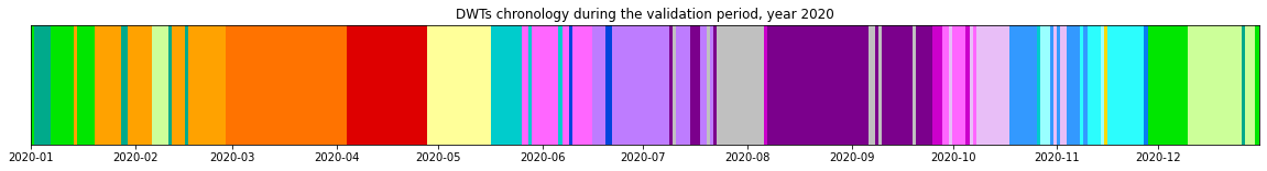
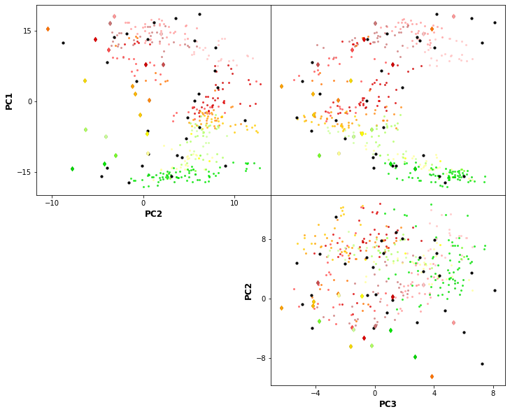
The resulting classification can be seen in the PCs space of the predictor index data. The obtained centroids (black dots), span the wide variability of the data.
Plot_scatter_kmeans(xds_kma_ord, val_bmus, xds_kma_ord.cenEOFs.values, figsize=(12,10));
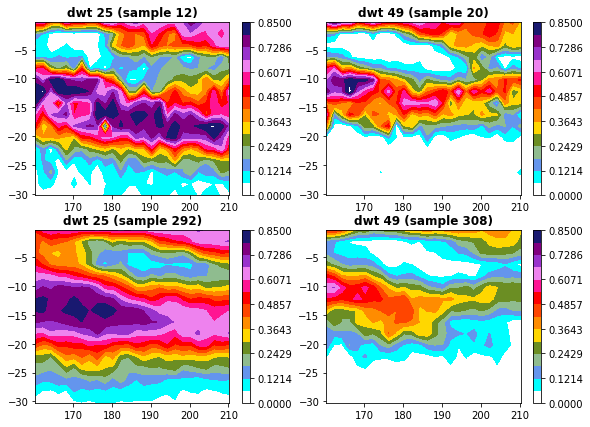
Cluster comparison#
Plot_bmus_comparison_validation_calibration(xs, xds_kma, xs_val, val_bmus, 25, 49);
Predictand computation and plotting#
From the DWT the daily expected mean number of TCs in 8x8º cells in the target area is known for each day and thus maps at different time scales can be computed.
Daily mean expected number of TCs
xds_timeline_val, xs_M_val = ds_monthly_probabilities(
    df_2021, val_bmus, xs_val,
    xds_count_tcs_8, xds_count_tcs_8_964,
)
print(xds_timeline_val)
<xarray.Dataset>
Dimensions:         (lat: 5, lon: 8, time: 366)
Coordinates:
  * time            (time) datetime64[ns] 2020-01-01 2020-01-02 ... 2020-12-31
  * lat             (lat) int64 -30 -22 -14 -6 2
  * lon             (lon) int64 160 168 176 184 192 200 208 216
Data variables:
    bmus            (time) int64 18 23 23 23 23 23 18 ... 15 23 15 15 15 18 15
    mask_tcs        (time) bool False False False False ... False False False
    id_tcs          (time) object nan nan nan nan nan ... nan nan nan nan nan
    counts_tcs      (time, lat, lon) float64 6.0 3.0 3.0 2.0 ... nan nan nan nan
    counts_tcs_964  (time, lat, lon) float64 1.0 1.0 nan nan ... nan nan nan nan
    probs_tcs       (time, lat, lon) float64 0.01942 0.009709 ... nan nan
    probs_tcs_964   (time, lat, lon) float64 0.003236 0.003236 nan ... nan nan
Monthly aggregated mean expected number of TCs
print(xs_M_val)
<xarray.Dataset>
Dimensions:         (lat: 5, lon: 8, time: 12)
Coordinates:
  * time            (time) datetime64[ns] 2020-01-01 2020-02-01 ... 2020-12-01
  * lat             (lat) int64 -30 -22 -14 -6 2
  * lon             (lon) int64 160 168 176 184 192 200 208 216
Data variables:
    mask_tcs        (time, lat, lon) float64 4.0 4.0 4.0 4.0 ... nan nan nan nan
    counts_tcs      (time, lat, lon) float64 110.0 111.0 82.0 ... nan nan nan
    counts_tcs_964  (time, lat, lon) float64 13.0 45.0 18.0 44.0 ... nan nan nan
    probs_tcs       (time, lat, lon) float64 0.388 0.4207 0.3044 ... nan nan nan
    probs_tcs_964   (time, lat, lon) float64 0.04207 0.1776 0.07361 ... nan nan
Plot_validation_year(df_2021, xs_M_val, xds_timeline_val, 35, lo_area, la_area);
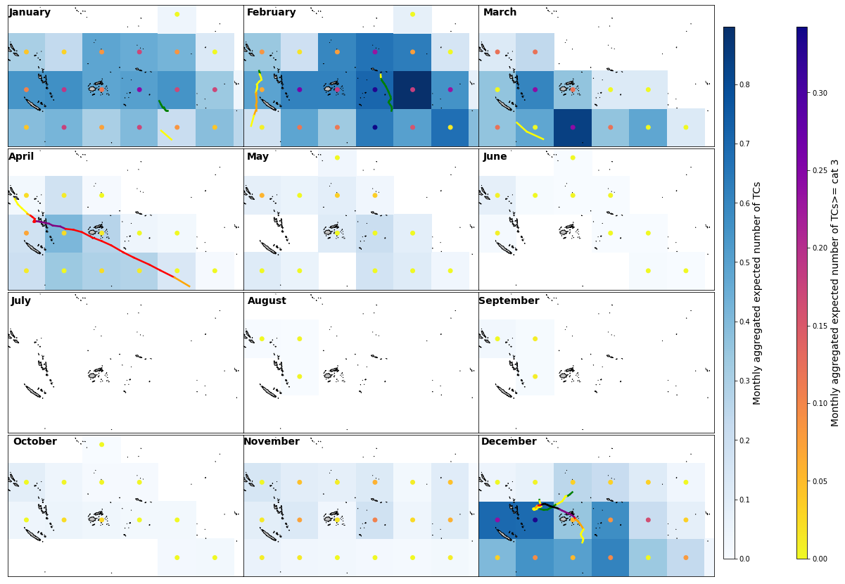
Whole period aggregated mean expected number of TCs
Plot_validation_full_season(df_2021, xs_M_val, xds_timeline_val, 35, lo_area, la_area);
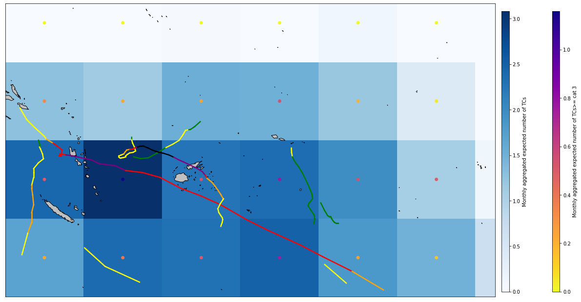
The model performs very well when estimating the expected TC activity (number and intensity of TCs), not understimating the threat.
In some cells adjacents to the cells including TC tracks it overstimates TC activity.