Seasonal Swells

This section contains the coding for automatically download 9-months forecast data from CFSR

from datetime import datetime

print("execution start: {0}".format(datetime.today().strftime('%Y-%m-%d %H:%M:%S')))

execution start: 2022-09-11 21:30:03

# common
import os
import os.path as op
import sys

# pip
import pickle as pk
import numpy as np
import xarray as xr
from IPython.core.display import HTML

# bluemath  
sys.path.insert(0, op.join(op.abspath(''), '..', '..'))
sys.path.insert(0, op.join(op.abspath(''), '..'))

from bluemath.ddviewer.downloader.forecast import download_prmsl, webscan_noaa_ncei
from bluemath.ddviewer.plotting.prmsl import plot_prmsl_seasonal

from bluemath.pca import spatial_gradient, dynamic_estela_predictor, standardise_predictor

from bluemath.plotting.forecast import Plot_monthly_mean, Plot_forecast_day_spec
from bluemath.plotting.teslakit import Plot_DWTs_Probs

# operational utils
from operational.util import clean_forecast_folder, read_config_args

Warning: ecCodes 2.21.0 or higher is recommended. You are running version 2.16.0

# hide warnings
import warnings
warnings.filterwarnings('ignore')

# HTML recipe to center notebook plots
HTML("""
<style>
.output_png {
    display: table-cell;
    text-align: center;
    vertical-align: middle;
}
</style>
""")

# matplotlib animatiom embed limit
import matplotlib
matplotlib.rcParams['animation.embed_limit'] = 2**128

Forecast parameteres

p_data = r'/media/administrador/HD2/SamoaTonga/data'

#site = 'Samoa'  # Samoa / Tongatapu

# (optional) get site from config file
nb_args = read_config_args(op.abspath(''), '04_seasonal_forecast_swells')
site = nb_args['site']

print('Study site: {0}'.format(site))
                           

Study site: Samoa

# automated forecast date, updated up to 3/4 days before present
years, months, days, runs = webscan_noaa_ncei()
year, month, day, _ = int(years[-1]), int(months[-1]), int(days[-1]), int(runs[-1])

print('last available date: {0:02}{1:02}{2:02}'.format(year, month, day))

last available date: 20220907

# get available run (NOAA prmsl forecast run  [0, 6, 12, 18])
runs = [int(r) for r in runs]

# selected run to solve
run_sel = runs[0]
print('run: {0}'.format(run_sel))

_clean_forecast_folder_days = 7  # days to keep after forecast folder cleaning

run: 0

# site related parameteres
pt_plot = []
if site == "Samoa":
    pt_plot = [187.93, -13.76]

elif site == "Tongatapu":
    pt_plot = [184.84, -21.21]

Database

# database
p_site = op.join(p_data, site)

# SLP
p_slp = op.join(p_data, 'SLP_hind_daily_wgrad.nc')

# deliverable folder
p_deliv = op.join(p_site, 'd04_seasonal_forecast_swells')

# estela
p_est = op.join(p_deliv, 'estela')
p_estela = op.join(p_est, 'estela.nc')

# estela pca 
p_pca_fit = op.join(p_est, 'PCA_fit.pkl')
p_pca_dyn = op.join(p_est, 'dynamic_predictor_PCA.nc')

# kma folder
p_kma = op.join(p_deliv, 'kma')

# estela slp kma
p_kma_slp_model = op.join(p_kma, 'slp_KMA_model.pkl')                   # KMeans model slp
p_kma_slp_classification = op.join(p_kma, 'slp_KMA_classification.nc')  # classified slp

# spectra kma
p_kma_spec_classification = op.join(p_kma, 'spec_KMA_classification.nc')   # classified superpoint

# conditioned probabilities
p_probs_cond = op.join(p_deliv, 'conditioned_prob_SLP_SPEC.nc')

# daily spectra
p_spec = op.join(p_deliv, 'spec')
p_sp_trans = op.join(p_spec, 'spec_daily_transformed_hs_t.nc')

Forecast Output folder

# output forecast folder
p_forecast = op.join(p_site, 'forecast', '04_seasonal_swells')

# forecast folder
date = '{0:04d}{1:02d}{2:02d}'.format(year, month, day)
p_fore_date = op.join(p_forecast, date)
print('forecast date code: {0}'.format(date))

# prepare forecast subfolders for this date
p_fore_dl = op.join(p_fore_date, 'download', 'mslp')

p_fore_prmsl = op.join(p_fore_date, 'prmsl')
p_fore_slp = op.join(p_fore_prmsl, 'slp.nc')
p_fore_pca_dy = op.join(p_fore_prmsl, 'dynamic_predictor.nc')
p_fore_slp_dy_f = op.join(p_fore_prmsl, 'slp_dy_f.nc')

for p in [p_fore_date, p_fore_dl, p_fore_prmsl]:
    if not op.isdir(p):
        os.makedirs(p)

# current month 
base_month = np.datetime64('{0:04d}-{1:02d}-{2:02d}'.format(year, month, day)).astype('datetime64[M]')

# clean forecast folder
clean_forecast_folder(p_forecast, days=_clean_forecast_folder_days)

forecast date code: 20220907
deleted folder:  /media/administrador/HD2/SamoaTonga/data/Samoa/forecast/04_seasonal_swells/20220820

Hindast data and estela for grid resampling

# load the slp with partitions
slp_h = xr.open_dataset(p_slp)
slp_h

<xarray.Dataset>
Dimensions:       (latitude: 67, longitude: 129, time: 15372)
Coordinates:
  * time          (time) datetime64[ns] 1979-01-01 1979-01-02 ... 2021-01-31
  * longitude     (longitude) float32 35.0 37.0 39.0 41.0 ... 287.0 289.0 291.0
  * latitude      (latitude) float32 66.0 64.0 62.0 60.0 ... -62.0 -64.0 -66.0
Data variables:
    slp           (time, latitude, longitude) float64 ...
    slp_gradient  (time, latitude, longitude) float64 ...

# load estela dataset
est = xr.open_dataset(p_estela, decode_times=False)

# prepare estela data
est = est.sel(time = 'ALL')
est = est.assign({'estela_mask':(('latitude', 'longitude'), np.where(est.F.values > 0, 1, np.nan))})

Download and process forecast SLP fields

Define the day and runs wanted for the download

Here we also preprocess the data for developing the dynamic predictor modified with travel time data from ESTELA

# download all prmsl runs
slp_run_list = []
pca_dy_run_list = []

for run in [run_sel]:
    
    # raw download
    slp_f = download_prmsl(year, month, day, run, p_f=p_fore_dl, load_local_cache=False, clean=True)
    
    # remove variables from dataset and rename slp and time
    slp_f = slp_f.drop(['time', 'meanSea', 'valid_time']).rename({'prmsl':'slp', 'ftime':'time'})
    
    # select slp area and resample to daily
    slp_f = slp_f.sel(longitude = slp_h.longitude, latitude = slp_h.latitude).resample(time='1D').mean()

    # calculate spatial gradient
    slp_f = spatial_gradient(slp_f, 'slp')

    # interpolate estela coordinates to downloaded slp
    est = est.sortby(est.latitude, ascending=False).interp(
        coords = {'latitude': slp_f.latitude, 'longitude': slp_f.longitude},
    )

    # get estela travel time and estela mask for slp data
    estela_D = est.drop('time').traveltime
    estela_mask = est.estela_mask
    
    # generate dynamic estela predictor
    pca_dy = dynamic_estela_predictor(slp_f, 'slp', estela_D)
    
    # assign "run" dimension to processed data
    slp_f = slp_f.expand_dims(dim='run').assign_coords({'run':(('run'), [run])})
    pca_dy = pca_dy.expand_dims(dim='run').assign_coords({'run':(('run'), [run])})
    
    # append to lists
    slp_run_list.append(slp_f)
    pca_dy_run_list.append(pca_dy)
    
# concatenate downloaded prmsl runs
slp_all = xr.concat(slp_run_list, dim = 'run')
pca_dy_all = xr.concat(pca_dy_run_list, dim = 'run')

# store data at forecast folder    
slp_all.to_netcdf(p_fore_slp)
pca_dy_all.to_netcdf(p_fore_pca_dy)

Downloading forecast data from:
https://www.ncei.noaa.gov/data/climate-forecast-system/access/operational-9-month-forecast/time-series/2022/202209/20220907/2022090700/prmsl.01.2022090700.daily.grb2
Storing local copy at:
/media/administrador/HD2/SamoaTonga/data/Samoa/forecast/04_seasonal_swells/20220907/download/mslp

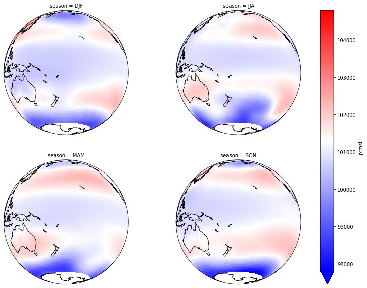
Forecast plotting by season

Figure Explanation

map with prmsl value by season.

# plot prmsl (seasonal)
plot_prmsl_seasonal(slp_all.rename({'slp': 'prmsl', 'time':'ftime'}).isel(run=0)); 

#.sel(run = run_sel));

Forecast

Transform slp from the validation period into the calibration PCA space:

# select dynamic predictor run
slp_dy_f = pca_dy_all.sel(run = run_sel).drop('run')
pos_i = np.where(np.isnan(slp_dy_f.max(dim=('longitude', 'latitude')).slp_comp.values)==False)[0][0]
slp_dy_f = slp_dy_f.isel(time = range(pos_i, len(slp_dy_f.time.values)))

# standardise estela predictor
d_pos, xds_norm = standardise_predictor(slp_dy_f, 'slp')

data_norm = xds_norm.pred_norm.values

# load estela pca and get PCs
pca_fit = pk.load(open(p_pca_fit, 'rb'))
PCs_f = pca_fit.transform(data_norm)

# load spectra kma 
spec_kma = xr.open_dataset(p_kma_spec_classification)
num_clusters_spec = len(np.unique(spec_kma.bmus))

Obtain SLP clusters where each day belongs to:

# load estela dynamic predictor PCA
slp_pcs = xr.open_dataset(p_pca_dyn)

# get PCs that explain 90% of the EV
n_percent = np.cumsum((slp_pcs.variance / np.sum(slp_pcs.variance))*100)
ev = 90
n_pcs = np.where(n_percent > ev)[0][0]
PCs_f = PCs_f[:, :n_pcs]

print('Number of PCs explaining ' + str(ev) + '% of the EV is: ' + str(n_pcs))

Number of PCs explaining 90% of the EV is: 521

# load slp kma
slp_kma = xr.open_dataset(p_kma_slp_classification)
num_clusters_slp = len(np.unique(slp_kma.bmus))

mask = np.where(np.isnan(slp_kma.est_mask) == True)
kma_fit = pk.load(open(p_kma_slp_model, "rb"))[0]

# intersect dates
c, i_sp, i_slp = np.intersect1d(spec_kma.time, slp_kma.time, return_indices=True)

slp_kma = slp_kma.isel(time = i_slp)
spec_kma = spec_kma.isel(time = i_sp)

# kma predict forecat PCs
bmus_slp_f = kma_fit.predict(PCs_f)

sorted_bmus = np.zeros((len(bmus_slp_f),),) * np.nan
for i in range(num_clusters_slp):
    posc = np.where(bmus_slp_f == slp_kma.kma_order[i].values)
    sorted_bmus[posc] = i

slp_dy_f['bmus'] = sorted_bmus

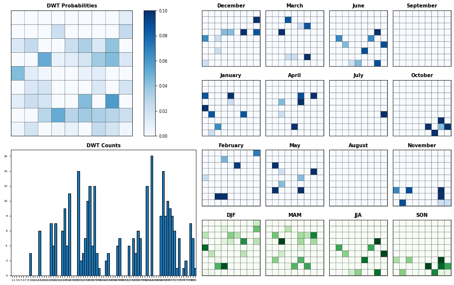
Seasonality of SLP clusters in the forecast period

Figure Explanation

SLP DWT clusters probabilities.
Upper left panel: Probability for each SLP DWT cluster
Lower left panel: Histogram of SLP DWT cluster occurences
Right panel: This panel displays each cluster probability for all months and seasons

Plot_DWTs_Probs(slp_dy_f.bmus.values+1, slp_dy_f.time.values, len(np.unique(slp_kma.bmus)));

Obtain the probability of each spectral cluster at the daily scale:

# load conditioned probabilities
cond_prob = xr.open_dataset(p_probs_cond)

p_f = np.full([len(cond_prob.ir), len(cond_prob.ic), len(slp_dy_f.time)], np.nan)

for a in range(len(slp_dy_f.time)):
    p_f[:, :, a] = cond_prob.prob_sp[:, :, slp_dy_f.bmus[a].values.astype('int')]

slp_dy_f['prob_spec'] = (('ir','ic','time'), p_f)

# store forecast
slp_dy_f.to_netcdf(p_fore_slp_dy_f)

Daily

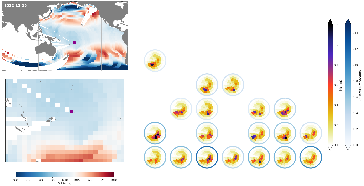
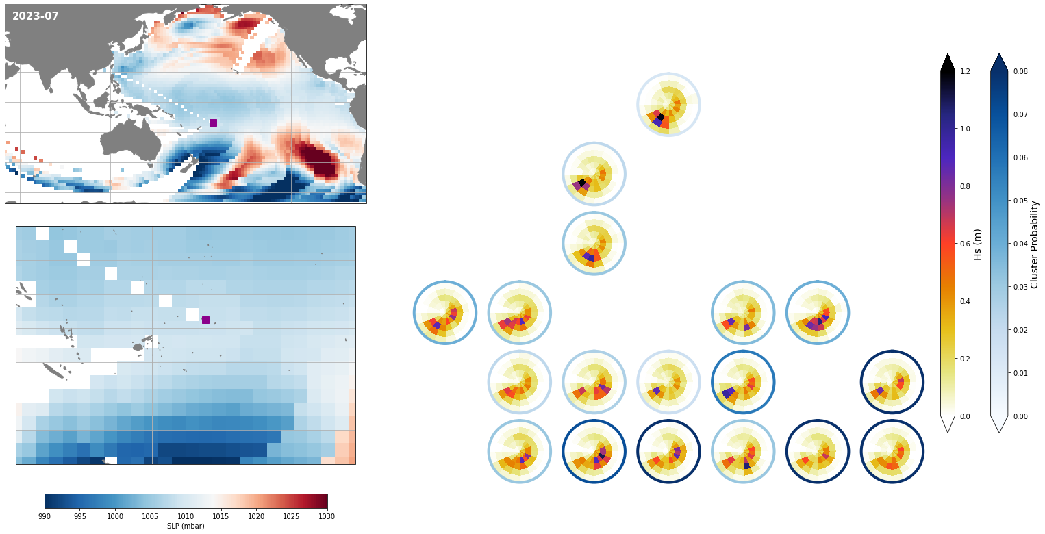
Each day, represented by one KMA cluster, has a specific distribution of different spectra probabilities

Figure Explanation

The figures below, both at the daily and monthly scale, have 3 different panels.
Upper left panel: SLP associated to that day
Lower left panel: Real spectra from the hindcast
Right panel: This panel displays only the clusters that are probable under those SLP conditions according to the model, where the blue line surrounding each spectrum has the information of the probability.

Figure Explanation

Also, the mean hindcast spectra and anomalies are shown below for comparison.
Mean model spectra is calculated as the sum of each cluster spectra multiplied by its probability of occurrence

# get some random day for plotting
plot_day_list = [np.random.choice(slp_dy_f.time.values)]

for day in plot_day_list:
    slp_d = slp_dy_f.sel(time=day)

    Plot_forecast_day_spec(
        slp_d, spec_kma, 
        mask = mask,
        extent = (50, 290, -67, 65), 
        extent_zoom = (160, 210, -35, 0),
        prob_min = 0, prob_max = 0.15,
        s_min = 990, s_max = 1030, 
        lw = 4, 
        pt = pt_plot,
        title = str(slp_d.time.values.astype('datetime64[D]')),
    );

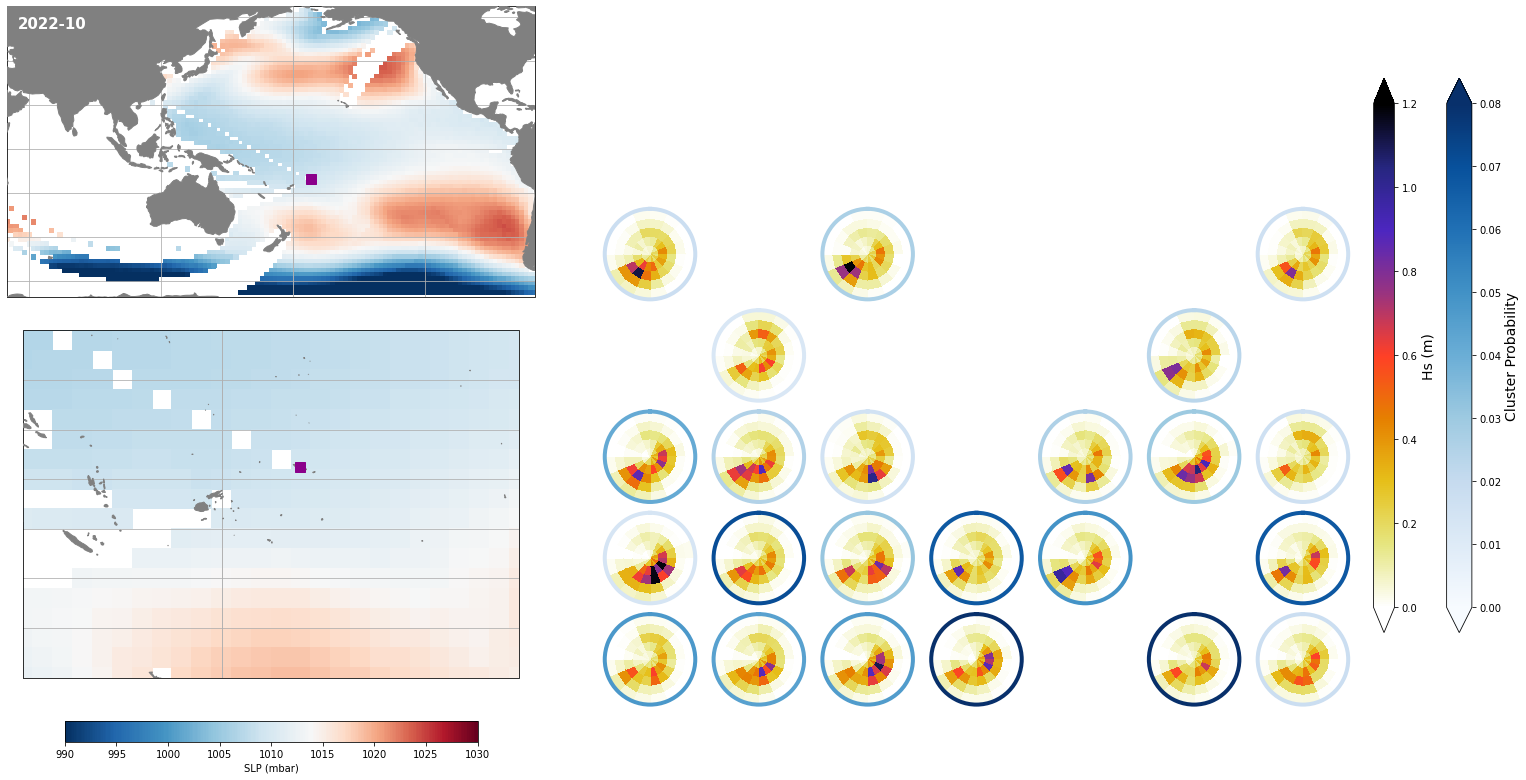
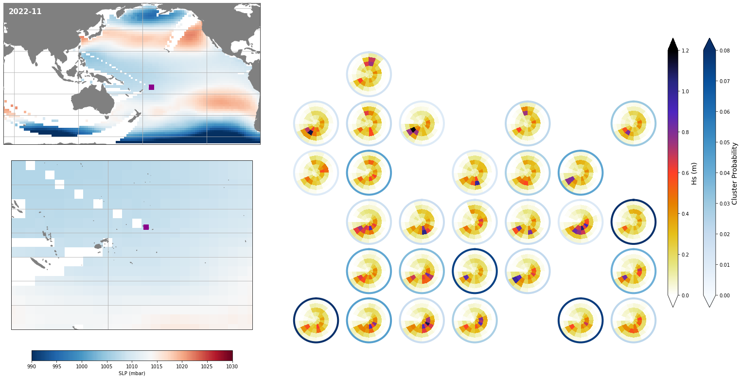
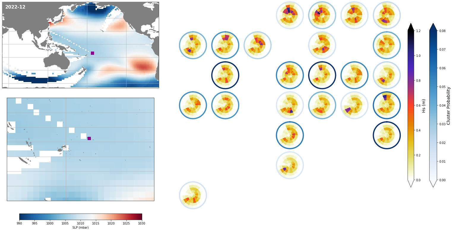
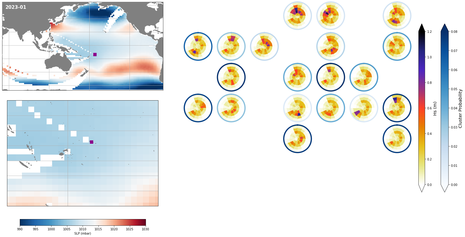
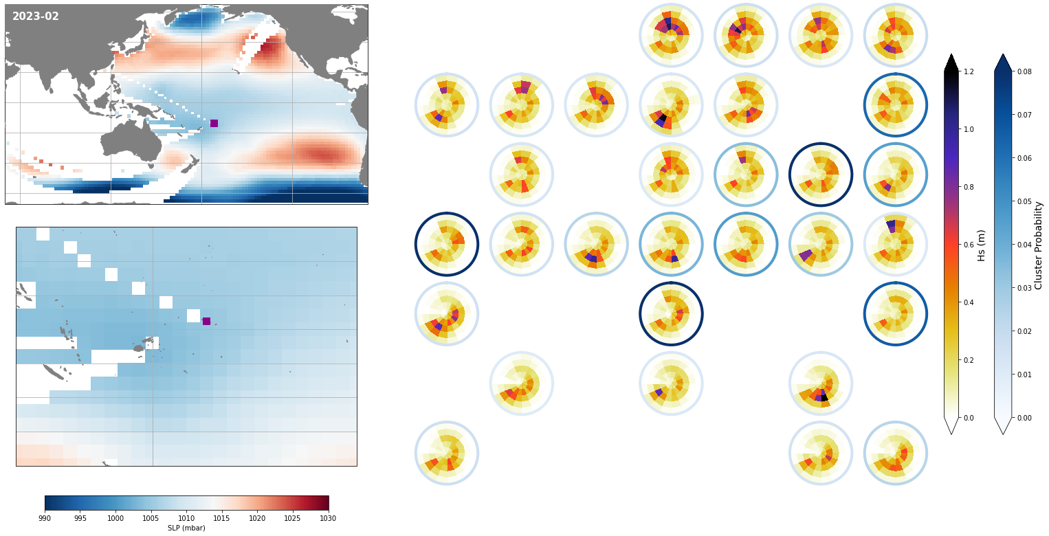
Monthly - Synoptic patterns

# monthly means
slp_dy_m = slp_dy_f.resample(time='1M',skipna=True).mean()

for month in slp_dy_m.time.dt.month.values:
    slp_m = slp_dy_m.isel(time = np.where(slp_dy_m.time.dt.month==month)[0]).isel(time=0)
    
    Plot_forecast_day_spec(
        slp_m, spec_kma, 
        extent = (50, 290, -67, 65),
        extent_zoom = (160, 210, -35, 0),
        prob_min = 0.03, prob_max = 0.08,
        s_min = 990, s_max = 1030,
        lw = 4,
        pt = pt_plot,
        title = str(slp_m.time.values.astype('datetime64[M]')),
    );

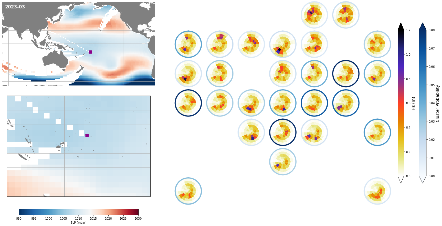
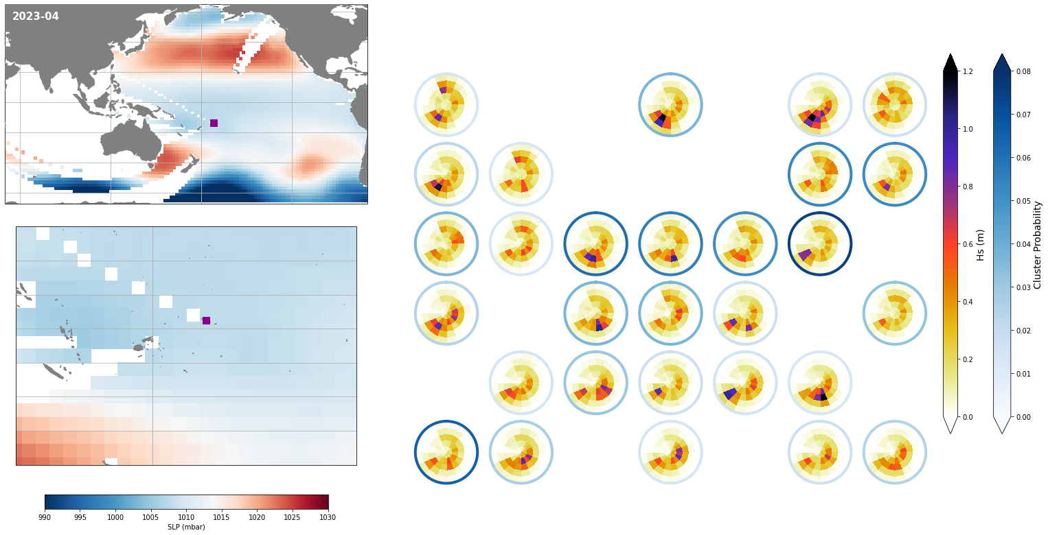
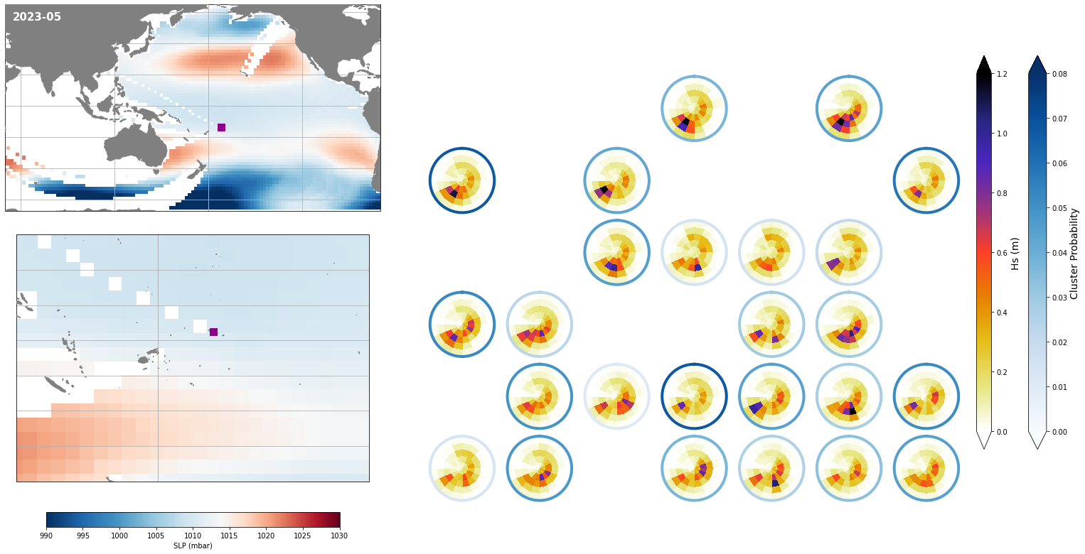
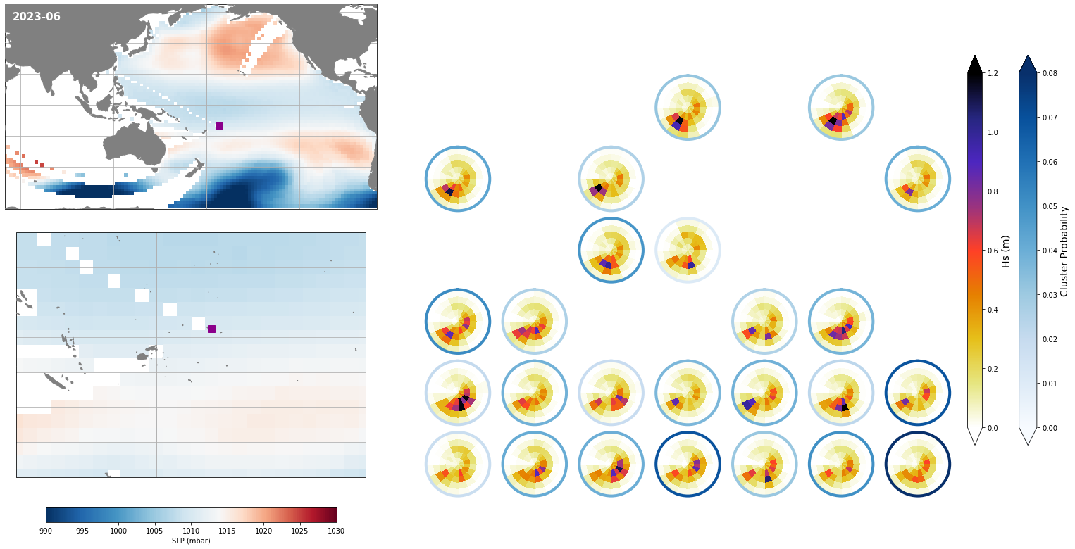
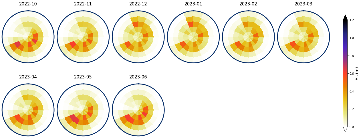
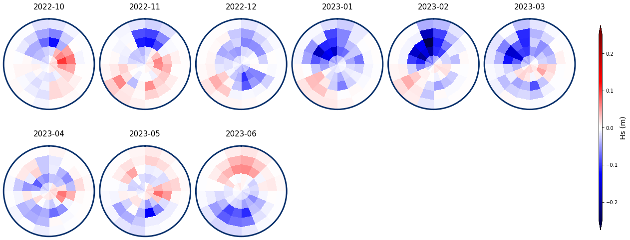
Monthly - Mean and anomalies

Figure Explanation

Here we show the results of the mean spectra and the anomalies associated to each of the 9 months.

# plot next 9 months after forecast date
list_months = [str(base_month + np.array(x+1, 'timedelta64[M]')) for x in range(9)]

Monthly means

# plot mean
Plot_monthly_mean(
    spec_kma, slp_dy_m,
    list_months,
    num_clus_pick = 49,
    perct_pick = [], 
    vmax = 1.2, vmin = 0,
    cmap = 'CMRmap_r',
    alpha_bk = 1,
);

We load the spec to calculate the mean for the anomalies

# load daily spectra
sp_mod_daily = xr.open_dataset(p_sp_trans)

# resample to monthly
spec_mod_m = sp_mod_daily.resample(time = '1M', skipna = True).mean()

Anomalies with respect to the mean specific month

# plot anomaly
Plot_monthly_mean(
    spec_kma, slp_dy_m,
    list_months,
    num_clus_pick = 49,
    perct_pick = [], 
    spec_mod_m = spec_mod_m,
    vmax = 0.25, vmin = -0.25,
    cmap = 'seismic',
    alpha_bk = 1,
);

print("execution end: {0}".format(datetime.today().strftime('%Y-%m-%d %H:%M:%S')))

execution end: 2022-09-11 21:30:51