Tailor-Made classification of large scale predictor
Contents
Tailor-Made classification of large scale predictor#
In this section, we are going to classify our tailor-made predictor (SLP fields and gradients modified using ESTELA) into a number of clusters (N=81) by reducing the dimensionality of the data by means of a principal component analysis (PCA) and then, performing a clustering of the PCs with the K-Means algorithm.
# common
import warnings
warnings.filterwarnings('ignore')

import os
import os.path as op
import sys
import pickle as pk

# pip
import numpy as np
import xarray as xr

# DEV: bluemath
sys.path.insert(0, op.join(op.abspath(''), '..', '..', '..', '..', '..'))

# bluemath modules
from bluemath.pca import dynamic_estela_predictor, PCA_EstelaPred
from bluemath.kma import kmeans_clustering_pcs

from bluemath.plotting.slp import Plot_slp_field, Plot_slp_kmeans
from bluemath.plotting.estela import Plot_estela
from bluemath.plotting.pca import Plot_EOFs_EstelaPred
from bluemath.plotting.teslakit import Plot_DWTs_Probs
Database and site parameters#
# database
p_data = r'/media/administrador/HD2/SamoaTonga/data'
site = 'Samoa'
p_site = op.join(p_data, site)

# SLP
p_slp = op.join(p_data, 'SLP_hind_daily_wgrad.nc')

# deliverable folder
p_deliv = op.join(p_site, 'd04_seasonal_forecast_swells')

# estela
p_est = op.join(p_deliv, 'estela')
p_estela = op.join(p_est, 'estela.nc')


# output files:

# dynamic predictor
p_dynp = op.join(p_est, 'dynamic_predictor.nc')

# PCA
p_pca_fit = op.join(p_est, 'PCA_fit.pkl')
p_pca_dyn = op.join(p_est, 'dynamic_predictor_PCA.nc')

# KMA
p_kma = op.join(p_deliv, 'kma')

p_kma_slp_model = op.join(p_kma, 'slp_KMA_model.pkl')                   # KMeans model
p_kma_slp_classification = op.join(p_kma, 'slp_KMA_classification.nc')  # classified SLP
# make output folders
for p in [p_kma]:
    if not op.isdir(p):
        os.makedirs(p)
# K-Means classification parameters
num_clusters = 81
min_data = 5
SLP data
# load the slp with partitions
slp = xr.open_dataset(p_slp)
PCA : Principal component analysis#
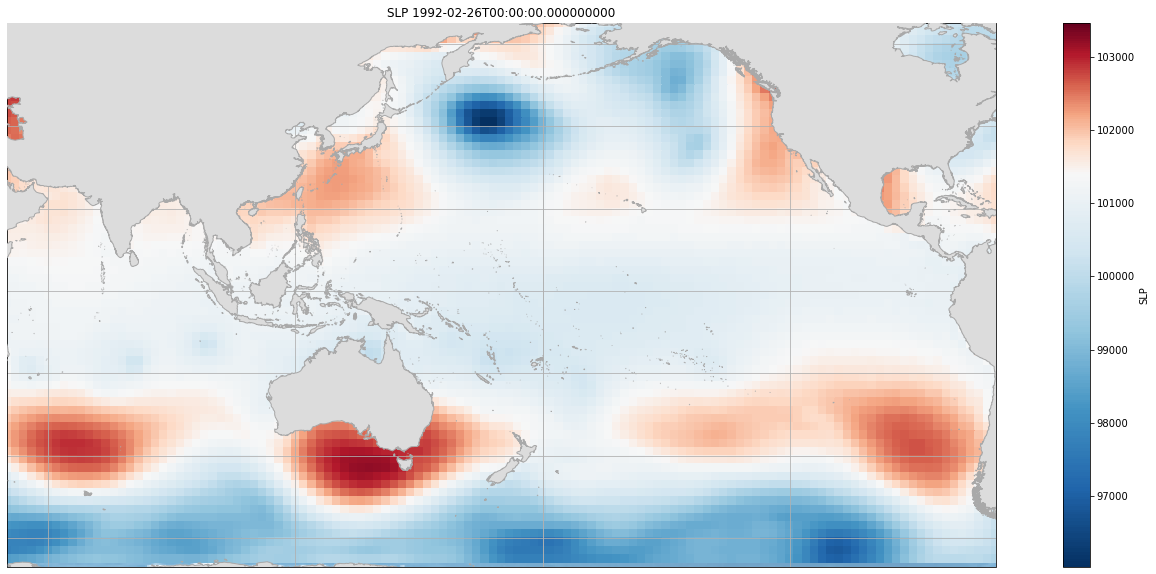
Area of SLP fields#
First, we define the area of influence, based on the wave generation area extracted from ESTELA
Here is an example for a given time, of the SLP area used for constructing the predictor.
Plot_slp_field(slp, extent = (50, 290, -67, 65), time = 4804);
Dynamic predictor#
The SLP and SLP gradient fields are modified to consider the travel time of swell waves, resulting on our Dynamic Predictor.
The dynamic predictor is constructed as follows:
\(P_t = \{...,{SLP}{t-i+1,\Omega i},{SLPG}{t-i+1,\Omega i}...\}\) for i=1,…,p
where Ωi represents the spatial domain between the daily isochrones i−1 and i, and p is the number of days of the last isochrone predicted by ESTELA, which represents the longest possible wave propagation time from generation until arrival at the target location.
ESTELA:
# load estela dataset
est = xr.open_dataset(p_estela, decode_times=False)

# prepare estela data
est = est.sel(time='ALL')
est = est.assign({'estela_mask':(('latitude','longitude'), np.where(est.F.values > 0, 1, np.nan))})
est = est.sortby(est.latitude, ascending = False).interp(
    coords = {
        'latitude' : slp.latitude,
        'longitude' : slp.longitude,
    }
)
estela_D = est.drop('time').traveltime
estela_mask = est.estela_mask  # mask for slp
Plot_estela(est, extent = (50, 290, -67, 65), figsize = [20, 8]);
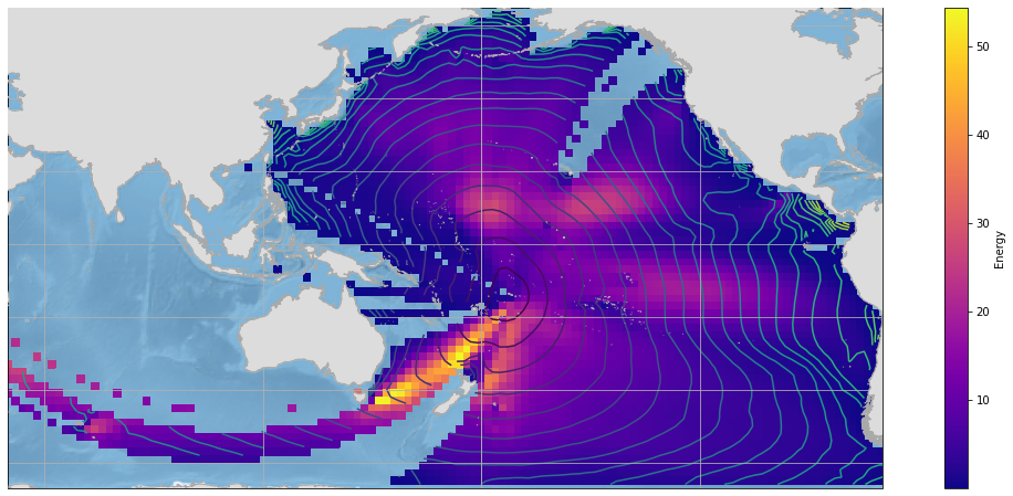
Then, we calculate the dynamic predictor with the information from the travel time extracted from ESTELA
# generate dynamic estela predictor
pca_dy = dynamic_estela_predictor(slp, 'slp', estela_D)
pca_dy.to_netcdf(p_dynp)

# load dynamic estela predictor
#pca_dy = xr.open_dataset(p_dynp)

pca_dy
<xarray.Dataset>
Dimensions:            (latitude: 67, longitude: 129, time: 15347)
Coordinates:
  * time               (time) datetime64[ns] 1979-01-26 ... 2021-01-31
  * latitude           (latitude) float32 66.0 64.0 62.0 ... -62.0 -64.0 -66.0
  * longitude          (longitude) float32 35.0 37.0 39.0 ... 287.0 289.0 291.0
Data variables:
    slp_comp           (time, latitude, longitude) float64 nan nan ... 1.001e+05
slp_gradient_comp (time, latitude, longitude) float64 nan nan ... 0.0 0.0- latitude: 67
- longitude: 129
- time: 15347
- time(time)datetime64[ns]1979-01-26 ... 2021-01-31
array(['1979-01-26T00:00:00.000000000', '1979-01-27T00:00:00.000000000', '1979-01-28T00:00:00.000000000', ..., '2021-01-29T00:00:00.000000000', '2021-01-30T00:00:00.000000000', '2021-01-31T00:00:00.000000000'], dtype='datetime64[ns]') - latitude(latitude)float3266.0 64.0 62.0 ... -64.0 -66.0
array([ 66., 64., 62., 60., 58., 56., 54., 52., 50., 48., 46., 44., 42., 40., 38., 36., 34., 32., 30., 28., 26., 24., 22., 20., 18., 16., 14., 12., 10., 8., 6., 4., 2., 0., -2., -4., -6., -8., -10., -12., -14., -16., -18., -20., -22., -24., -26., -28., -30., -32., -34., -36., -38., -40., -42., -44., -46., -48., -50., -52., -54., -56., -58., -60., -62., -64., -66.], dtype=float32) - longitude(longitude)float3235.0 37.0 39.0 ... 289.0 291.0
array([ 35.,  37.,  39.,  41.,  43.,  45.,  47.,  49.,  51.,  53.,  55.,  57.,
        59.,  61.,  63.,  65.,  67.,  69.,  71.,  73.,  75.,  77.,  79.,  81.,
        83.,  85.,  87.,  89.,  91.,  93.,  95.,  97.,  99., 101., 103., 105.,
       107., 109., 111., 113., 115., 117., 119., 121., 123., 125., 127., 129.,
       131., 133., 135., 137., 139., 141., 143., 145., 147., 149., 151., 153.,
       155., 157., 159., 161., 163., 165., 167., 169., 171., 173., 175., 177.,
       179., 181., 183., 185., 187., 189., 191., 193., 195., 197., 199., 201.,
       203., 205., 207., 209., 211., 213., 215., 217., 219., 221., 223., 225.,
       227., 229., 231., 233., 235., 237., 239., 241., 243., 245., 247., 249.,
       251., 253., 255., 257., 259., 261., 263., 265., 267., 269., 271., 273.,
       275., 277., 279., 281., 283., 285., 287., 289., 291.], dtype=float32)
- slp_comp(time, latitude, longitude)float64nan nan nan ... 1.001e+05 1.001e+05
array([[[ nan, nan, nan, ..., nan, nan, nan], [ nan, nan, nan, ..., nan, nan, nan], [ nan, nan, nan, ..., nan, nan, nan], ..., [ nan, nan, nan, ..., 98670.20703125, 98841.37890625, 99049.99707031], [ nan, nan, nan, ..., 99097.87890625, 99264.53450521, 99148.75227865], [ nan, nan, nan, ..., 99399.44466146, 99411.17382812, 99432.68522135]], [[ nan, nan, nan, ..., nan, nan, nan], [ nan, nan, nan, ..., nan, nan, nan], [ nan, nan, nan, ..., nan, nan, nan], ... [ nan, nan, nan, ..., 100480.68847656, 100612.57779948, 100700.3515625 ], [ nan, nan, nan, ..., 100194.60188802, 100358.10807292, 98705.18684896], [ nan, nan, nan, ..., 98768.37890625, 98497.13704427, 98308.98144531]], [[ nan, nan, nan, ..., nan, nan, nan], [ nan, nan, nan, ..., nan, nan, nan], [ nan, nan, nan, ..., nan, nan, nan], ..., [ nan, nan, nan, ..., 99134.1813151 , 99263.25748698, 99397.75585938], [ nan, nan, nan, ..., 98700.79166667, 98865.69466146, 100448.97786458], [ nan, nan, nan, ..., 99922.3421224 , 100079.42578125, 100148.09765625]]]) - slp_gradient_comp(time, latitude, longitude)float64nan nan nan nan ... 0.0 0.0 0.0 0.0
array([[[            nan,             nan,             nan, ...,
                     nan,             nan,             nan],
        [            nan,             nan,             nan, ...,
                     nan,             nan,             nan],
        [            nan,             nan,             nan, ...,
                     nan,             nan,             nan],
        ...,
        [            nan,             nan,             nan, ...,
         218036.51282083, 265588.61098138,      0.        ],
        [            nan,             nan,             nan, ...,
         340386.43050428, 384733.07949873,      0.        ],
        [            nan,             nan,             nan, ...,
              0.        ,      0.        ,      0.        ]],

       [[            nan,             nan,             nan, ...,
                     nan,             nan,             nan],
        [            nan,             nan,             nan, ...,
                     nan,             nan,             nan],
        [            nan,             nan,             nan, ...,
                     nan,             nan,             nan],
...
        [            nan,             nan,             nan, ...,
         209019.58867816, 140476.240157  ,      0.        ],
        [            nan,             nan,             nan, ...,
         254374.57032324, 162252.99079573,      0.        ],
        [            nan,             nan,             nan, ...,
              0.        ,      0.        ,      0.        ]],

       [[            nan,             nan,             nan, ...,
                     nan,             nan,             nan],
        [            nan,             nan,             nan, ...,
                     nan,             nan,             nan],
        [            nan,             nan,             nan, ...,
                     nan,             nan,             nan],
        ...,
        [            nan,             nan,             nan, ...,
         312130.11788394, 290750.94028972,      0.        ],
        [            nan,             nan,             nan, ...,
         267533.49322446, 262869.87904194,      0.        ],
        [            nan,             nan,             nan, ...,
              0.        ,      0.        ,      0.        ]]])
PCA#
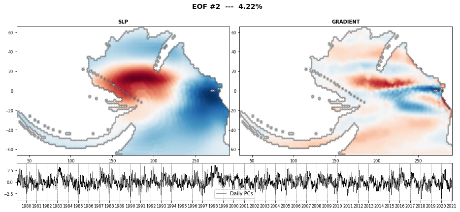
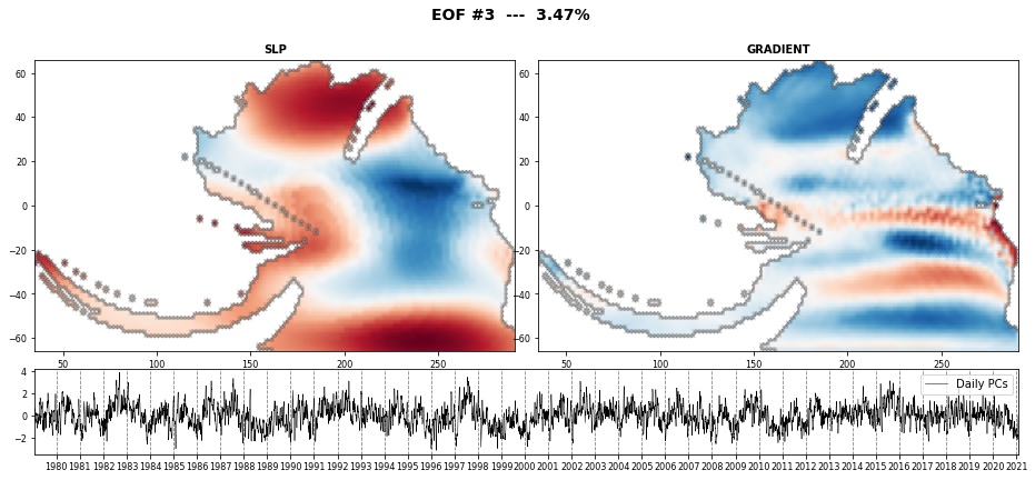
The PCA is used to reduce the high dimensionality of the original data space and thus, simplify the classification process, transforming the SLP predictor fields into a number of spatial modes with an associated temporal variability over time.
PCA projects the original data on a new space searching for the maximum variance of the sample data.
The eigenvectors (the empirical orthogonal functions, EOFs) of the data covariance matrix define the vectors of the new space.
They represent the spatial variability.
# PCA estela predictor
[pca, ipca] = PCA_EstelaPred(pca_dy, 'slp')

# store PCA fit
with open(p_pca_fit, 'wb') as fW:
    pk.dump(ipca, fW)

# store dynamic predictor PCA
pca.to_netcdf(p_pca_dyn)


# load PCA
#pca = xr.open_dataset(p_pca_dyn)
#ipca = pk.load(open(p_pca_fit, 'rb'))


# set pred_time as a coordinate
PCs = pca.assign_coords({'time': (('time'), pca.pred_time.values)}).PCs

# select slp at PCA predictor time
slp = slp.sel(time = pca.pred_time)
Here we select the PCs explaining 90% of the variance
ev = 90

n_percent = np.cumsum((pca.variance / np.sum(pca.variance)) * 100)
n_pcs = np.where(n_percent > ev)[0][0]

print('Number of PCs explaining ' + str(ev) + '% of the EV is: ' + str(n_pcs))
print('Number of PCs explaining {0}% of the EV is: {1}'.format(ev, n_pcs))
Number of PCs explaining 90% of the EV is: 521
Number of PCs explaining 90% of the EV is: 521
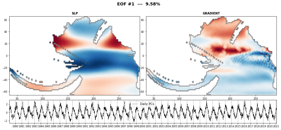
The eigenvectors (the empirical orthogonal functions, EOFs) of the data covariance matrix define the vectors of the new space.
They represent the spatial variability.
# plot first PCA EOFs

n_pcs_plot = 3

Plot_EOFs_EstelaPred(pca, n_pcs_plot, show=True, mask_land=[]);
K-MEANS Clustering#
Daily synoptic patterns are obtained using the K-means clustering algorithm. It divides the data space into 81 clusters, a number that which must be a compromise between an easy handle characterization of the synoptic patterns and the best reproduction of the variability in the data space. Previous works with similar anlaysis confirmed that the selection of this number is adequate (Rueda et al. 2017).
Each cluster is defined by a prototype and formed by the data for which the prototype is the nearest.
Finally the best match unit (bmus) of daily clusters are reordered into a lattice following a geometric criteria, so that similar clusters are placed next to each other for a more intuitive visualization.
# KMeans clustering for slp data
kma, kma_order, bmus, sorted_bmus, centers = kmeans_clustering_pcs(
    PCs, n_pcs,
    num_clusters,
    min_data,
    kma_tol = 0.0001,
    kma_n_init = 10,
)

# store kma output
pk.dump([kma, kma_order, bmus, sorted_bmus, centers], open(p_kma_slp_model, 'wb'))

# load kma
#kma, kma_order, bmus, sorted_bmus, centers = pk.load(open(p_kma_slp_model, 'rb'))
Iteration: 422
Number of sims: 152
Minimum number of data: 5
# add KMA data to SLP
slp['bmus'] = ('time', sorted_bmus)
slp['kma_order'] = kma_order
slp['cluster'] = np.arange(num_clusters)
slp['centers'] = (('cluster', 'dims'), centers)

# add estela mask to SLP
slp['est_mask'] = (('latitude','longitude'), estela_mask.values)

# store updated dataset
slp.to_netcdf(p_kma_slp_classification)
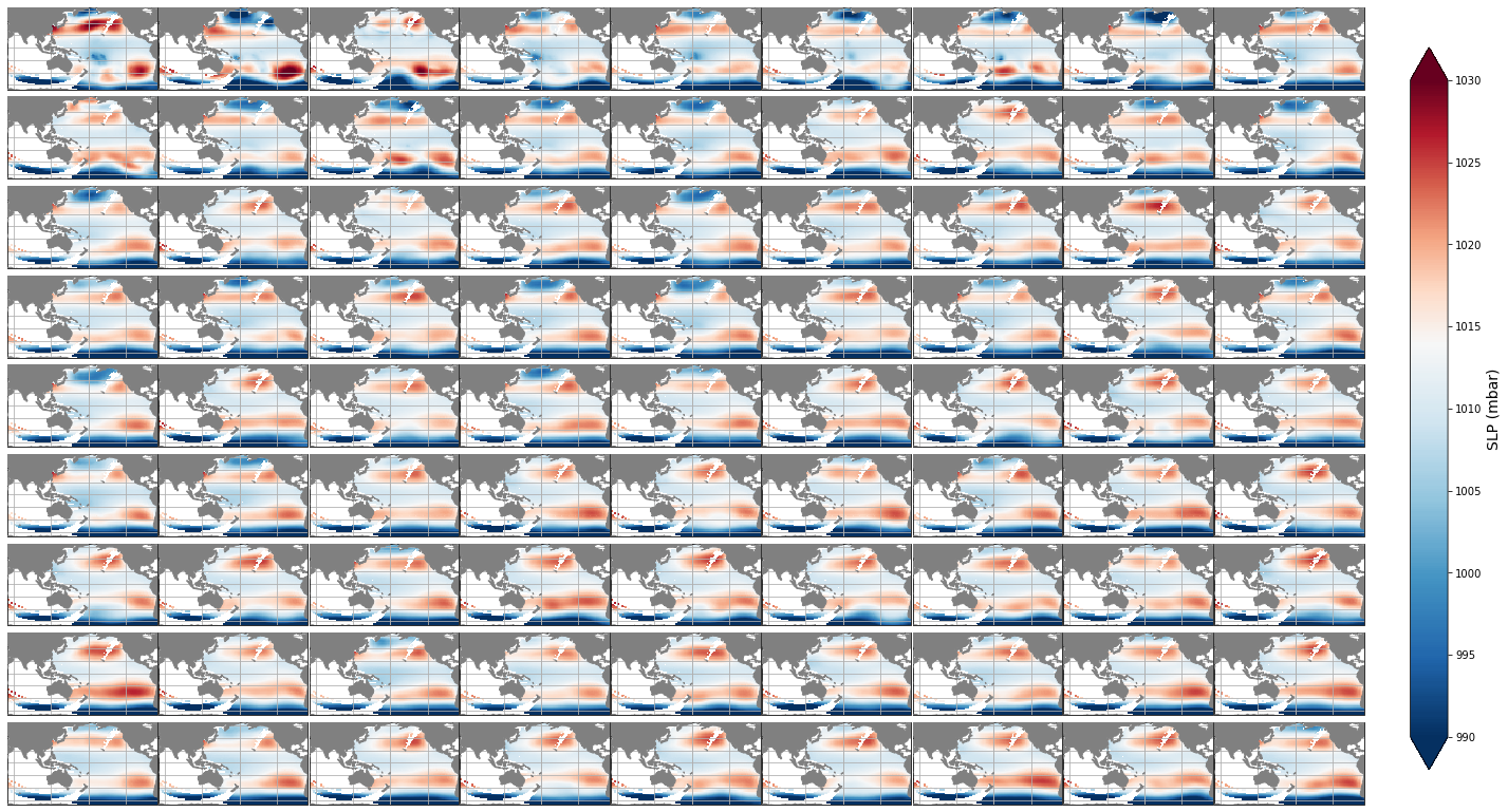
Mean#
The mean SLP associated to each of the different clusters is shown below.
Plot_slp_kmeans(slp, extent=(50, 290, -67, 65), figsize=[23,14]);
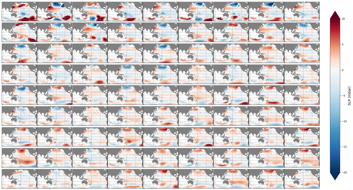
Anomaly#
The SLP anomaly with respect to the mean and associated to each of the different clusters is shown below.
Plot_slp_kmeans(slp, extent=(50, 290, -67, 65), figsize=[23,14], anomaly=True);
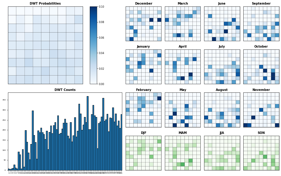
Seasonality#
Probability of each KMA cluster, conditioned to each month and season
Plot_DWTs_Probs(slp.bmus+1, pca.pred_time.values, num_clusters, vmax=0.1);