Statistical Model Validation
Contents
Statistical Model Validation#
For the validation of the model, we split the time into a calibration period: (1979-2015) and validation period: (2016-2021)
In the validation period, the results of the model can be compared to the real spectra, providing insights on the performance of the statistical model.
Important
The predictor and predictand classification developed in this section is only used for validating the statistical model. As this section is the repetition of the process presented in previous sections, here only some of the figures are shown for simplicity
# common
import warnings
warnings.filterwarnings('ignore')

import os
import os.path as op
import sys

# pip
import pickle as pk
import numpy as np
import xarray as xr
from sklearn.decomposition import PCA

# DEV: bluemath
sys.path.insert(0, op.join(op.abspath(''), '..', '..', '..', '..', '..'))

# bluemath modules
from bluemath.binwaves.spectra import set_t_h, group_bins_dir_t
from bluemath.binwaves.plotting.classification import Plot_spectra_hs_pcs, Plot_kmeans_clusters_hs
from bluemath.binwaves.plotting.classification import Plot_specs_hs_inside_cluster, Plot_kmeans_clusters_probability

from bluemath.pca import dynamic_estela_predictor, PCA_EstelaPred, standardise_predictor
from bluemath.kma import kmeans_clustering_pcs, calculate_conditioned_probabilities

from bluemath.plotting.slp import Plot_slp_field, Plot_slp_kmeans
from bluemath.plotting.teslakit import Plot_DWTs_Probs, Plot_Probs_WT_WT
from bluemath.plotting.validation import Plot_validation_spec, Plot_daily_mean, Plot_entropy, calculate_entropy, Plot_prob_comparison
Database and site parameters#
# database
p_data = r'/media/administrador/HD2/SamoaTonga/data'
site = 'Samoa'
p_site = op.join(p_data, site)

# SLP
p_slp = op.join(p_data, 'SLP_hind_daily_wgrad.nc')

# deliverable folder
p_deliv = op.join(p_site, 'd04_seasonal_forecast_swells')

# spectra data
p_spec = op.join(p_deliv, 'spec')

# superpoint
p_superpoint = op.join(p_spec, 'super_point_superposition.nc')

# daily spectrum
p_sp_trans = op.join(p_spec, 'spec_daily_transformed_hs_t.nc')

# estela
p_est = op.join(p_deliv, 'estela')
p_estela = op.join(p_est, 'estela.nc')


# validation files:
p_valid = op.join(p_deliv, 'validation')
p_valid_est = op.join(p_valid, 'estela')

# dynamic predictor
p_dynp = op.join(p_valid_est, 'dynamic_predictor.nc')

# PCA
p_pca_slp_fit = op.join(p_valid_est, 'PCA_slp_fit.pkl')
p_pca_dyn = op.join(p_valid_est, 'dynamic_predictor_PCA.nc')

p_pca_spec_fit = op.join(p_valid_est, 'PCA_spec_fit.pkl')

# KMA
p_valid_kma = op.join(p_valid, 'kma')

p_kma_slp_model = op.join(p_valid_kma, 'slp_KMA_model.pkl')                     # KMeans model SLP
p_kma_slp_classification = op.join(p_valid_kma, 'slp_KMA_classification.nc')    # classified SLP

p_kma_spec_model = op.join(p_valid_kma, 'spec_KMA_model.pkl')                   # KMeans model spectra
p_kma_spec_classification = op.join(p_valid_kma, 'spec_KMA_classification.nc')  # classified superpoint

# conditioned probabilities
p_probs_cond = op.join(p_valid, 'conditioned_prob_SLP_SPEC.nc')
# generate validation data folders
for p in [p_valid, p_valid_est, p_valid_kma]:
    if not op.isdir(p):
        os.makedirs(p)
# validation training time period
time_train_1 = '1979-01-01'
time_train_2 = '2015-12-31'

# validation test time period
time_test_1 = '2016-01-01'
time_test_2 = '2020-12-31'

# K-Means classification parameters - SLP
num_clusters_slp = 81
min_data_slp = 5

# K-Means classification parameters
num_clusters_spec = 49
min_data_frac_spec = 10  # to calculate minimum number of data for each cluster
Classification of Tailor-made large scale predictor (1979-2015)#
# load the slp with partitions
slp = xr.open_dataset(p_slp)
# select training time period
slp = slp.sel(time = slice(time_train_1, time_train_2))
PCA : Principal component analysis#
Estela:
# load estela dataset
est = xr.open_dataset(p_estela, decode_times=False)

# prepare estela data
est = est.sel(time = 'ALL')
est = est.assign({'estela_mask': (('latitude', 'longitude'), np.where(est.F.values > 0, 1, np.nan))})
est = est.sortby(est.latitude,ascending=False).interp(
    coords = {
        'latitude': slp.latitude,
        'longitude': slp.longitude,
    },
)
estela_D = est.drop('time').traveltime
estela_mask = est.estela_mask # mask for slp
Dynamic predictor:
# generate dynamic estela predictor
pca_dy = dynamic_estela_predictor(slp, 'slp', estela_D)
pca_dy.to_netcdf(p_dynp)


# load dynamic estela predictor
#pca_dy = xr.open_dataset(p_dynp)

pca_dy
<xarray.Dataset>
Dimensions:            (latitude: 67, longitude: 129, time: 13489)
Coordinates:
  * time               (time) datetime64[ns] 1979-01-26 ... 2015-12-31
  * latitude           (latitude) float32 66.0 64.0 62.0 ... -62.0 -64.0 -66.0
  * longitude          (longitude) float32 35.0 37.0 39.0 ... 287.0 289.0 291.0
Data variables:
    slp_comp           (time, latitude, longitude) float64 nan nan ... 9.981e+04
slp_gradient_comp (time, latitude, longitude) float64 nan nan ... 0.0 0.0- latitude: 67
- longitude: 129
- time: 13489
- time(time)datetime64[ns]1979-01-26 ... 2015-12-31
array(['1979-01-26T00:00:00.000000000', '1979-01-27T00:00:00.000000000', '1979-01-28T00:00:00.000000000', ..., '2015-12-29T00:00:00.000000000', '2015-12-30T00:00:00.000000000', '2015-12-31T00:00:00.000000000'], dtype='datetime64[ns]') - latitude(latitude)float3266.0 64.0 62.0 ... -64.0 -66.0
array([ 66., 64., 62., 60., 58., 56., 54., 52., 50., 48., 46., 44., 42., 40., 38., 36., 34., 32., 30., 28., 26., 24., 22., 20., 18., 16., 14., 12., 10., 8., 6., 4., 2., 0., -2., -4., -6., -8., -10., -12., -14., -16., -18., -20., -22., -24., -26., -28., -30., -32., -34., -36., -38., -40., -42., -44., -46., -48., -50., -52., -54., -56., -58., -60., -62., -64., -66.], dtype=float32) - longitude(longitude)float3235.0 37.0 39.0 ... 289.0 291.0
array([ 35.,  37.,  39.,  41.,  43.,  45.,  47.,  49.,  51.,  53.,  55.,  57.,
        59.,  61.,  63.,  65.,  67.,  69.,  71.,  73.,  75.,  77.,  79.,  81.,
        83.,  85.,  87.,  89.,  91.,  93.,  95.,  97.,  99., 101., 103., 105.,
       107., 109., 111., 113., 115., 117., 119., 121., 123., 125., 127., 129.,
       131., 133., 135., 137., 139., 141., 143., 145., 147., 149., 151., 153.,
       155., 157., 159., 161., 163., 165., 167., 169., 171., 173., 175., 177.,
       179., 181., 183., 185., 187., 189., 191., 193., 195., 197., 199., 201.,
       203., 205., 207., 209., 211., 213., 215., 217., 219., 221., 223., 225.,
       227., 229., 231., 233., 235., 237., 239., 241., 243., 245., 247., 249.,
       251., 253., 255., 257., 259., 261., 263., 265., 267., 269., 271., 273.,
       275., 277., 279., 281., 283., 285., 287., 289., 291.], dtype=float32)
- slp_comp(time, latitude, longitude)float64nan nan nan ... 9.995e+04 9.981e+04
array([[[ nan, nan, nan, ..., nan, nan, nan], [ nan, nan, nan, ..., nan, nan, nan], [ nan, nan, nan, ..., nan, nan, nan], ..., [ nan, nan, nan, ..., 98670.20703125, 98841.37890625, 99049.99707031], [ nan, nan, nan, ..., 99097.87890625, 99264.53450521, 99148.75227865], [ nan, nan, nan, ..., 99399.44466146, 99411.17382812, 99432.68522135]], [[ nan, nan, nan, ..., nan, nan, nan], [ nan, nan, nan, ..., nan, nan, nan], [ nan, nan, nan, ..., nan, nan, nan], ... [ nan, nan, nan, ..., 100426.47884115, 100266.31640625, 100105.37988281], [ nan, nan, nan, ..., 100261.31152344, 100100.18294271, 99389.65950521], [ nan, nan, nan, ..., 99584.21061198, 99442.74544271, 99351.50911458]], [[ nan, nan, nan, ..., nan, nan, nan], [ nan, nan, nan, ..., nan, nan, nan], [ nan, nan, nan, ..., nan, nan, nan], ..., [ nan, nan, nan, ..., 101104.01595052, 101013.69401042, 100914.52213542], [ nan, nan, nan, ..., 100915.63769531, 100826.92089844, 99935.01204427], [ nan, nan, nan, ..., 100101.88671875, 99949.31575521, 99812.74707031]]]) - slp_gradient_comp(time, latitude, longitude)float64nan nan nan nan ... 0.0 0.0 0.0 0.0
array([[[            nan,             nan,             nan, ...,
                     nan,             nan,             nan],
        [            nan,             nan,             nan, ...,
                     nan,             nan,             nan],
        [            nan,             nan,             nan, ...,
                     nan,             nan,             nan],
        ...,
        [            nan,             nan,             nan, ...,
         218036.51282083, 265588.61098138,      0.        ],
        [            nan,             nan,             nan, ...,
         340386.43050428, 384733.07949873,      0.        ],
        [            nan,             nan,             nan, ...,
              0.        ,      0.        ,      0.        ]],

       [[            nan,             nan,             nan, ...,
                     nan,             nan,             nan],
        [            nan,             nan,             nan, ...,
                     nan,             nan,             nan],
        [            nan,             nan,             nan, ...,
                     nan,             nan,             nan],
...
        [            nan,             nan,             nan, ...,
         135533.50482238, 141416.05971297,      0.        ],
        [            nan,             nan,             nan, ...,
         152804.43929539, 163714.31516014,      0.        ],
        [            nan,             nan,             nan, ...,
              0.        ,      0.        ,      0.        ]],

       [[            nan,             nan,             nan, ...,
                     nan,             nan,             nan],
        [            nan,             nan,             nan, ...,
                     nan,             nan,             nan],
        [            nan,             nan,             nan, ...,
                     nan,             nan,             nan],
        ...,
        [            nan,             nan,             nan, ...,
          56607.74374821,  65464.18838694,      0.        ],
        [            nan,             nan,             nan, ...,
          74692.67568838,  80329.62836515,      0.        ],
        [            nan,             nan,             nan, ...,
              0.        ,      0.        ,      0.        ]]])
PCA:
# PCA estela predictor
[pca, ipca] = PCA_EstelaPred(pca_dy, 'slp')

# store PCA fit
with open(p_pca_slp_fit, 'wb') as fW:
    pk.dump(ipca, fW)

# store dynamic predictor PCA
pca.to_netcdf(p_pca_dyn)


# load PCA
#pca = xr.open_dataset(p_pca_dyn)
#ipca = pk.load(open(p_pca_slp_fit, 'rb'))


# set pred_time as a coordinate
PCs = pca.assign_coords({'time': (('time'), pca.pred_time.values)}).PCs

# select slp at PCA predictor time
slp = slp.sel(time = pca.pred_time)
ev = 90

n_percent = np.cumsum((pca.variance / np.sum(pca.variance)) * 100)
n_pcs = np.where(n_percent > ev)[0][0]
n_pcs_slp = n_pcs

print('Number of PCs explaining ' + str(ev) + '% of the EV is: ' + str(n_pcs))
print('Number of PCs explaining {0}% of the EV is: {1}'.format(ev, n_pcs))
Number of PCs explaining 90% of the EV is: 510
Number of PCs explaining 90% of the EV is: 510
K-MEANS Clustering#
We define 81 synoptic weather types by means of the K-Means clustering algorithm
# KMeans clustering for SLP data
kma, kma_order, bmus, sorted_bmus, centers = kmeans_clustering_pcs(
    PCs, n_pcs,
    num_clusters_slp,
    min_data_slp,
    kma_tol = 0.0001,
    kma_n_init = 10,
)

# store kma output
pk.dump([kma, kma_order, bmus, sorted_bmus, centers], open(p_kma_slp_model, 'wb'))

# load kma
#kma, kma_order, bmus, sorted_bmus, centers = pk.load(open(p_kma_slp_model, 'rb'))
Iteration: 844
Number of sims: 61
Minimum number of data: 7
# add KMA data to SLP
slp['bmus'] = ('time', sorted_bmus)
slp['kma_order'] = kma_order
slp['cluster'] = np.arange(num_clusters_slp)
slp['centers'] = (('cluster', 'dims'), centers)

# add estela mask to SLP
slp['est_mask'] = (('latitude','longitude'), estela_mask.values)

# store updated dataset
slp.to_netcdf(p_kma_slp_classification)
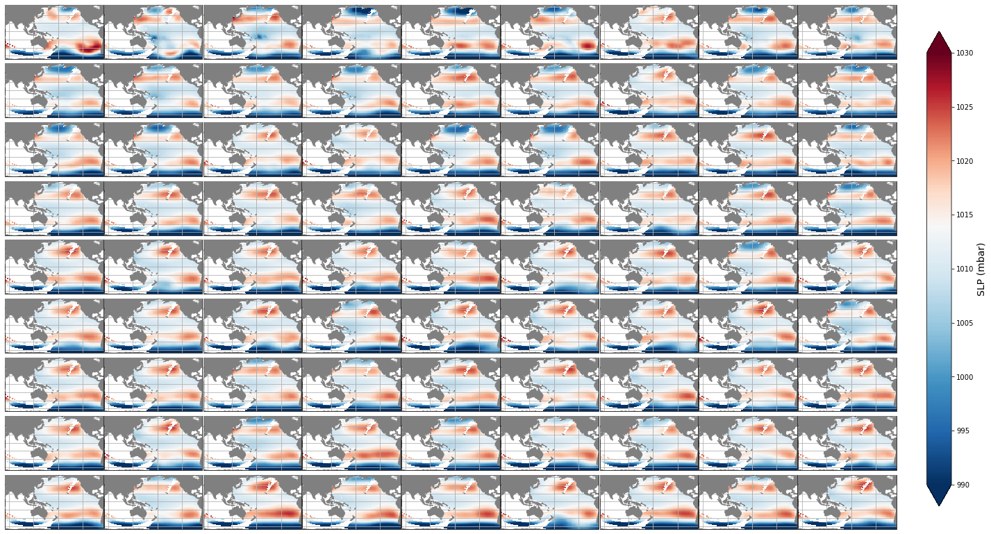
The mean SLP associated to each of the different clusters is shown below.
Plot_slp_kmeans(slp, extent=(50, 290, -67, 65), figsize=[23,14]);
Classification of spectra (1979-2015)#
# Load superpoint
sp = xr.open_dataset(p_superpoint)
print(sp)
<xarray.Dataset>
Dimensions:  (dir: 24, freq: 29, time: 366477)
Coordinates:
  * time     (time) datetime64[ns] 1979-01-01 1979-01-01T01:00:00 ... 2020-10-01
  * dir      (dir) float32 262.5 247.5 232.5 217.5 ... 322.5 307.5 292.5 277.5
  * freq     (freq) float32 0.035 0.0385 0.04235 ... 0.4171 0.4589 0.5047
Data variables:
    efth     (time, freq, dir) float64 ...
    Wspeed   (time) float32 ...
    Wdir     (time) float32 ...
    Depth    (time) float32 ...
# calculate and add t and h to superpoint
sp = set_t_h(sp)
# select training time period
sp = sp.sel(time=slice(time_train_1, time_train_2))
Transform and group in bins
# group spectra data by direction and period bins
dir_bins = np.linspace(0.0, 360.0, 17)
t_bins = np.arange(0.0, 30, 5)

sp_mod = group_bins_dir_t(sp, dir_bins, t_bins)
sp_mod
<xarray.Dataset>
Dimensions:   (dir_bins: 16, t_bins: 5, time: 324779)
Coordinates:
  * t_bins    (t_bins) object (0.0, 5.0] (5.0, 10.0] ... (20.0, 25.0]
  * dir_bins  (dir_bins) object (0.0, 22.5] (22.5, 45.0] ... (337.5, 360.0]
  * time      (time) datetime64[ns] 1979-01-01 ... 2015-12-31T23:00:00
Data variables:
    h         (t_bins, dir_bins, time) float64 0.0 3.113e-05 ... 2.547e-07
    dir       (dir_bins) float64 22.5 45.0 67.5 90.0 ... 292.5 315.0 337.5 360.0
    t         (t_bins) float64 5.0 10.0 15.0 20.0 25.0
h_t (t_bins, dir_bins, time) float64 0.0 0.02232 ... 0.001867 0.002019- dir_bins: 16
- t_bins: 5
- time: 324779
- t_bins(t_bins)object(0.0, 5.0] ... (20.0, 25.0]
array([Interval(0.0, 5.0, closed='right'), Interval(5.0, 10.0, closed='right'), Interval(10.0, 15.0, closed='right'), Interval(15.0, 20.0, closed='right'), Interval(20.0, 25.0, closed='right')], dtype=object) - dir_bins(dir_bins)object(0.0, 22.5] ... (337.5, 360.0]
array([Interval(0.0, 22.5, closed='right'), Interval(22.5, 45.0, closed='right'), Interval(45.0, 67.5, closed='right'), Interval(67.5, 90.0, closed='right'), Interval(90.0, 112.5, closed='right'), Interval(112.5, 135.0, closed='right'), Interval(135.0, 157.5, closed='right'), Interval(157.5, 180.0, closed='right'), Interval(180.0, 202.5, closed='right'), Interval(202.5, 225.0, closed='right'), Interval(225.0, 247.5, closed='right'), Interval(247.5, 270.0, closed='right'), Interval(270.0, 292.5, closed='right'), Interval(292.5, 315.0, closed='right'), Interval(315.0, 337.5, closed='right'), Interval(337.5, 360.0, closed='right')], dtype=object) - time(time)datetime64[ns]1979-01-01 ... 2015-12-31T23:00:00
array(['1979-01-01T00:00:00.000000000', '1979-01-01T01:00:00.000000000',
       '1979-01-01T02:00:00.000000000', ..., '2015-12-31T21:00:00.000000000',
       '2015-12-31T22:00:00.000000000', '2015-12-31T23:00:00.000000000'],
      dtype='datetime64[ns]')
- h(t_bins, dir_bins, time)float640.0 3.113e-05 ... 2.547e-07
array([[[0.00000000e+00, 3.11349244e-05, 3.11910083e-04, ..., 2.66953251e-03, 2.78026336e-03, 2.89604586e-03], [0.00000000e+00, 1.80685423e-06, 1.33951845e-05, ..., 2.21515800e-04, 2.48259195e-04, 2.75985925e-04], [0.00000000e+00, 7.58283830e-07, 6.98746678e-07, ..., 1.10629365e-04, 1.09257003e-04, 1.11056920e-04], ..., [0.00000000e+00, 5.14713811e-05, 1.17267312e-04, ..., 1.20112840e-03, 1.22315853e-03, 1.29208152e-03], [0.00000000e+00, 1.41668210e-04, 6.01923627e-04, ..., 4.15855313e-03, 4.30557292e-03, 4.49600377e-03], [0.00000000e+00, 4.64471265e-05, 2.51691087e-04, ..., 2.38724068e-03, 2.47166196e-03, 2.55886900e-03]], [[0.00000000e+00, 7.11408997e-31, 2.02724002e-16, ..., 6.27996723e-03, 6.21043064e-03, 6.19092203e-03], [0.00000000e+00, 5.08657380e-31, 6.11422932e-17, ..., 3.19417233e-03, 3.00456347e-03, 2.83061113e-03], [0.00000000e+00, 0.00000000e+00, 4.37325344e-29, ..., 8.75397197e-03, 8.18081079e-03, 7.70860963e-03], ... [0.00000000e+00, 0.00000000e+00, 0.00000000e+00, ..., 4.34036596e-03, 3.77340698e-03, 3.28649258e-03], [0.00000000e+00, 0.00000000e+00, 0.00000000e+00, ..., 3.98193846e-03, 3.39467507e-03, 2.87533710e-03], [0.00000000e+00, 0.00000000e+00, 0.00000000e+00, ..., 9.34211396e-03, 9.21041065e-03, 9.05994399e-03]], [[0.00000000e+00, 0.00000000e+00, 0.00000000e+00, ..., 3.47124276e-06, 2.71205556e-06, 2.08742015e-06], [0.00000000e+00, 0.00000000e+00, 0.00000000e+00, ..., 3.54657824e-07, 3.33411991e-07, 3.09417847e-07], [0.00000000e+00, 0.00000000e+00, 0.00000000e+00, ..., 4.09101605e-10, 3.54223988e-10, 3.72251068e-10], ..., [0.00000000e+00, 0.00000000e+00, 0.00000000e+00, ..., 7.15747299e-08, 4.92836721e-08, 3.59095089e-08], [0.00000000e+00, 0.00000000e+00, 0.00000000e+00, ..., 2.61439075e-05, 4.24236935e-05, 6.56504459e-05], [0.00000000e+00, 0.00000000e+00, 0.00000000e+00, ..., 2.10637804e-07, 2.17963797e-07, 2.54672623e-07]]]) - dir(dir_bins)float6422.5 45.0 67.5 ... 337.5 360.0
array([ 22.5, 45. , 67.5, 90. , 112.5, 135. , 157.5, 180. , 202.5, 225. , 247.5, 270. , 292.5, 315. , 337.5, 360. ]) - t(t_bins)float645.0 10.0 15.0 20.0 25.0
array([ 5., 10., 15., 20., 25.])
- h_t(t_bins, dir_bins, time)float640.0 0.02232 ... 0.001867 0.002019
array([[[0.00000000e+00, 2.23194711e-02, 7.06439051e-02, ...,
         2.06670076e-01, 2.10912811e-01, 2.15259689e-01],
        [0.00000000e+00, 5.37677111e-03, 1.46397730e-02, ...,
         5.95336274e-02, 6.30249721e-02, 6.64512965e-02],
        [0.00000000e+00, 3.48317977e-03, 3.34364275e-03, ...,
         4.20721979e-02, 4.18104299e-02, 4.21534188e-02],
        ...,
        [0.00000000e+00, 2.86974232e-02, 4.33160131e-02, ...,
         1.38629197e-01, 1.39894733e-01, 1.43782142e-01],
        [0.00000000e+00, 4.76097821e-02, 9.81365275e-02, ...,
         2.57947378e-01, 2.62467458e-01, 2.68208986e-01],
        [0.00000000e+00, 2.72608515e-02, 6.34591002e-02, ...,
         1.95437588e-01, 1.98863248e-01, 2.02341058e-01]],

       [[0.00000000e+00, 3.37380260e-15, 5.69524717e-08, ...,
         3.16984977e-01, 3.15225142e-01, 3.14729650e-01],
        [0.00000000e+00, 2.85280881e-15, 3.12774150e-08, ...,
         2.26068037e-01, 2.19255594e-01, 2.12813952e-01],
        [0.00000000e+00, 0.00000000e+00, 2.64522315e-14, ...,
         3.74250653e-01, 3.61791338e-01, 3.51194752e-01],
...
        [0.00000000e+00, 0.00000000e+00, 0.00000000e+00, ...,
         2.63525815e-01, 2.45712254e-01, 2.29311756e-01],
        [0.00000000e+00, 0.00000000e+00, 0.00000000e+00, ...,
         2.52410411e-01, 2.33055361e-01, 2.14488680e-01],
        [0.00000000e+00, 0.00000000e+00, 0.00000000e+00, ...,
         3.86618447e-01, 3.83883537e-01, 3.80734952e-01]],

       [[0.00000000e+00, 0.00000000e+00, 0.00000000e+00, ...,
         7.45250858e-03, 6.58732791e-03, 5.77916278e-03],
        [0.00000000e+00, 0.00000000e+00, 0.00000000e+00, ...,
         2.38212619e-03, 2.30967354e-03, 2.22501361e-03],
        [0.00000000e+00, 0.00000000e+00, 0.00000000e+00, ...,
         8.09050412e-05, 7.52833568e-05, 7.71752362e-05],
        ...,
        [0.00000000e+00, 0.00000000e+00, 0.00000000e+00, ...,
         1.07013816e-03, 8.87997046e-04, 7.57992178e-04],
        [0.00000000e+00, 0.00000000e+00, 0.00000000e+00, ...,
         2.04524453e-02, 2.60533893e-02, 3.24099851e-02],
        [0.00000000e+00, 0.00000000e+00, 0.00000000e+00, ...,
         1.83581177e-03, 1.86746372e-03, 2.01860397e-03]]])
Resample to daily values
# resample spectra to daily
sp_mod_daily = sp_mod.resample(time = '1D').mean()
sp_mod_daily = sp_mod_daily.assign_coords(
    t_bins = sp_mod_daily.t.values[0,:],
    dir_bins = sp_mod_daily.dir.values[0,:],
)

# drop t and dir variables
sp_mod_daily = sp_mod_daily.drop(['t', 'dir'])

# TODO guardar spec_daily_transformed_hs_t ??
PCA : Principal component analysis#
m = np.full((len(sp_mod_daily.time), len(sp_mod_daily.dir_bins) * len(sp_mod_daily.t_bins)), 0.000001)
for ti in range(m.shape[0]):
    m[ti, :] = np.ravel(sp_mod_daily.h_t.isel(time = ti).values)
p = 95  # Explained variance

ipca = PCA(n_components = np.shape(m)[1])

# add PCA data to superpoint
sp_mod_daily['PCs'] =  (('time','pc'), ipca.fit_transform(m))
sp_mod_daily['EOFs'] = (('pc','components'), ipca.components_)
sp_mod_daily['pc'] =   range(np.shape(m)[1])
sp_mod_daily['EV'] =   (('pc'), ipca.explained_variance_)

APEV = np.cumsum(sp_mod_daily.EV.values) / np.sum(sp_mod_daily.EV.values) * 100.0
n_pcs = np.where(APEV > p)[0][0]
sp_mod_daily['n_pcs'] = n_pcs
n_pcs_spec = n_pcs

print('Number of PCs explaining {0}% of the EV is: {1}'.format(p, n_pcs))

# store PCA
pk.dump(ipca, open(p_pca_spec_fit, "wb"))
Number of PCs explaining 95% of the EV is: 24
K-MEANS Clustering#
# minimun data for each cluster
min_data_spec = np.int(len(sp_mod_daily.time) / num_clusters_spec / min_data_frac_spec)

# KMeans clustering for spectral data
kma, kma_order, bmus, sorted_bmus, centers = kmeans_clustering_pcs(
    sp_mod_daily.PCs.values[:], n_pcs,
    num_clusters_spec,
    min_data = min_data_spec,
    kma_tol = 0.000001,
    kma_n_init = 10,
)

# store kma output
pk.dump([kma, kma_order, bmus, sorted_bmus, centers], open(p_kma_spec_model, 'wb'))

#kma, kma_order, bmus, sorted_bmus, centers = pk.load(open(p_kma_spec_model, 'rb'))
Iteration: 974
Number of sims: 125
Minimum number of data: 32
# add KMA data to superpoint
sp_mod_daily['kma_order'] =  kma_order
sp_mod_daily['n_pcs'] =  n_pcs
sp_mod_daily['bmus'] = (('time'), sorted_bmus)
sp_mod_daily['centroids'] = (('clusters', 'n_pcs_'), centers)
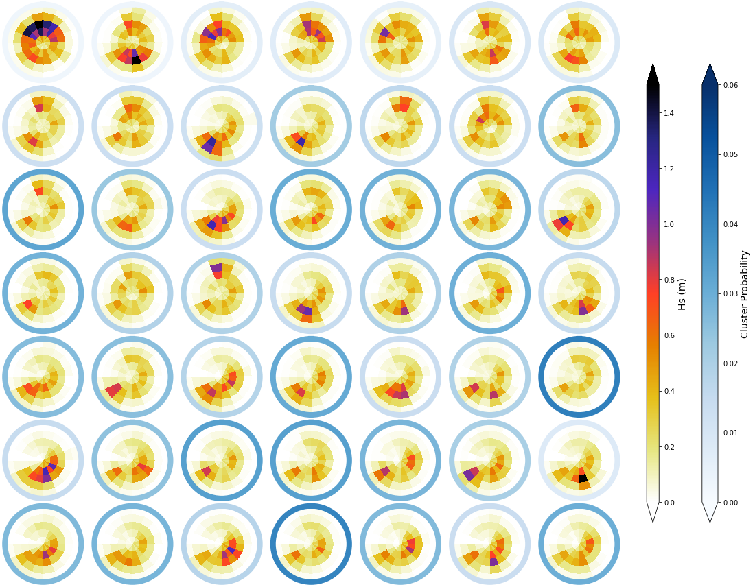
_, mean_h_clust, hs_m = Plot_kmeans_clusters_hs(sp_mod_daily,  vmax=1.5);

# add mean to superpoint h dataset
sp_mod_daily['clusters'] = range(num_clusters_spec)
sp_mod_daily['Mean_h'] = (('t_bins','dir_bins','clusters'), mean_h_clust)
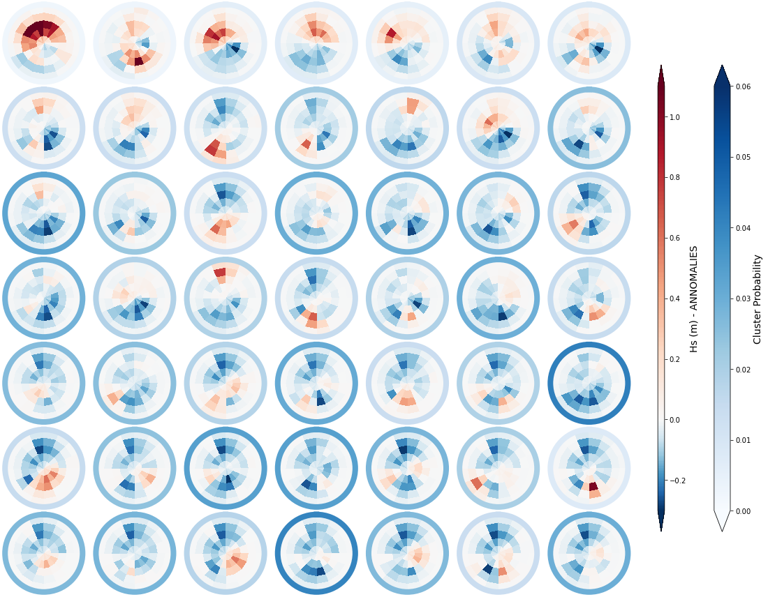
_, annomalies_h_clust, hs_an = Plot_kmeans_clusters_hs(sp_mod_daily, annomaly = True, vmax=1.1);

# add annomaly to superpoint dataset
sp_mod_daily['Annomaly_h'] = (('t_bins','dir_bins','clusters'), annomalies_h_clust)
sp_mod_daily.to_netcdf(p_kma_spec_classification)
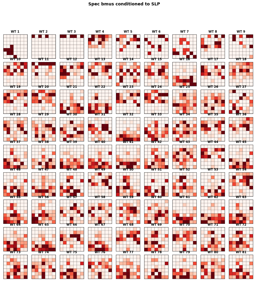
Conditioned probabilities (1979-2015)#
The figure below represents the conditioned probability of the 49 predictand clusters, conditioned to the 81 predictor clusters.
We observe large variability on the probability distributions of spectral clusters associated to each SLP cluster.
c, i_sp, i_slp = np.intersect1d(sp_mod_daily.time, slp.time, return_indices=True)

slp = slp.isel(time = i_slp)
sp_mod_daily = sp_mod_daily.isel(time = i_sp)
num_clusters_slp = len(np.unique(slp.bmus))
num_clusters_sp = len(np.unique(sp_mod_daily.bmus))

f3 = Plot_Probs_WT_WT(
    slp.bmus, sp_mod_daily.bmus,
    num_clusters_slp, num_clusters_sp,
    wt_colors = False,
    ttl = 'Spec bmus conditioned to SLP',
    figsize = [15,15],
    vmax = 0.07,
);
# calculate conditioned probabilities
conditioned_prob = calculate_conditioned_probabilities(slp, num_clusters_slp, sp_mod_daily, num_clusters_sp)

conditioned_prob.to_netcdf(p_probs_cond)
Validation 2016-2021#
The validation period corresponds to the years from 2016-2021, which were not included in the calibration process
Obtain SLP cluster and Spec probabilities for each day#
Here, we are projecting the SLP fields from the validation period into the PCA calibration space to obtain the SLP cluster that characterizes each day
SLP fields for the validation period:
# load the slp with partitions
slp = xr.open_dataset(p_slp)
# select training time period
slp = slp.sel(time = slice(time_test_1, time_test_2))
Constructing the dynamic predictor:
slp_dy = dynamic_estela_predictor(slp, 'slp', estela_D)
Transform slp from the validation period into the calibration PCA space:
# standardise estela predictor
d_pos, xds_norm = standardise_predictor(slp_dy, 'slp')
data_norm = xds_norm.pred_norm.values

# load estela pca and get PCs
pca_fit = pk.load(open(p_pca_slp_fit, 'rb'))
PCs_2020 = pca_fit.transform(data_norm)
# load estela dynamic predictor PCA
slp_pcs = xr.open_dataset(p_pca_dyn)

# get PCs that explain 90% of the EV
#n_percent = np.cumsum((slp_pcs.variance / np.sum(slp_pcs.variance))*100)
#ev=90
#n_pcs=np.where(n_percent>ev)[0][0]
#print('Number of PCs explaining ' + str(ev) + '% of the EV is: ' + str(n_pcs))

PCs_2020 = PCs_2020[:, :n_pcs_slp]
Obtain SLP clusters where each day belongs to:
# load slp kma
slp_kma = xr.open_dataset(p_kma_slp_classification)
num_clusters_slp = len(np.unique(slp_kma.bmus))

mask = np.where(np.isnan(slp_kma.est_mask) == True)
kma_fit = pk.load(open(p_kma_slp_model, "rb"))[0]
# kma predict validation PCs
bmus_slp = kma_fit.predict(PCs_2020)

sorted_bmus = np.zeros((len(bmus_slp),),) * np.nan
for i in range(num_clusters_slp):
    posc = np.where(bmus_slp == slp_kma.kma_order[i].values)
    sorted_bmus[posc] = i

slp_dy['bmus'] = sorted_bmus
Obtain the probability of each spectral cluster at the daily scale:
spec_kma = xr.open_dataset(p_kma_spec_classification)

num_clusters_spec = len(np.unique(spec_kma.bmus))
# Intersect dates
c, i_sp, i_slp = np.intersect1d(spec_kma.time, slp_kma.time, return_indices=True)

slp_kma = slp_kma.isel(time=i_slp)
spec_kma = spec_kma.isel(time=i_sp)
# load conditioned probabilities
cond_prob = xr.open_dataset(p_probs_cond)

p_f = np.full([len(cond_prob.ir), len(cond_prob.ic), len(slp_dy.time)], np.nan)

for a in range(len(slp_dy.time)):
    p_f[:, :, a] = cond_prob.prob_sp[:, :, slp_dy.bmus[a].values.astype('int')]

slp_dy['prob_spec'] = (('ir', 'ic', 'time'), p_f)
slp_dy['bmus'] = ('time', slp_dy.bmus)
Load spectral hindcast for comparison:
# spectral hindcast
sp_mod_daily = xr.open_dataset(p_sp_trans)
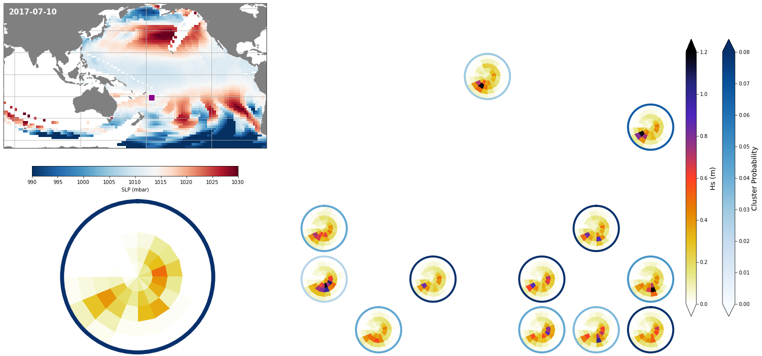
Results at the daily scale#
Each day, represented by one KMA cluster, has a specific distribution of different spectra probabilities
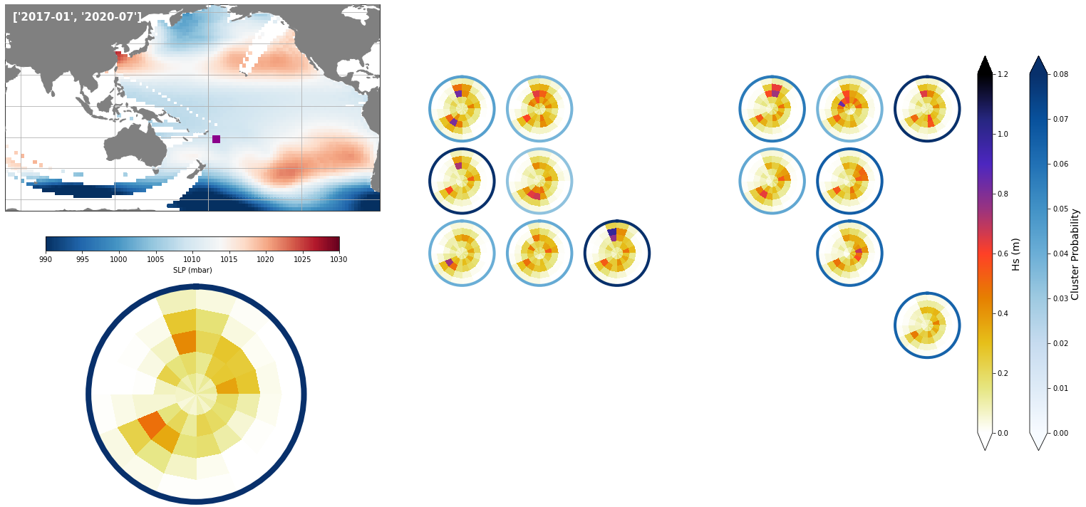
Figure Explanation
The figures below, both at the daily and monthly scale, have 3 different panels.
Upper left panel: SLP associated to that day
Lower left panel: Real spectra from the hindcast
Right panel: This panel displays only the clusters that are probable under those SLP conditions according to the model, where the blue line surrounding each spectrum has the information of the probability.
Figure Explanation
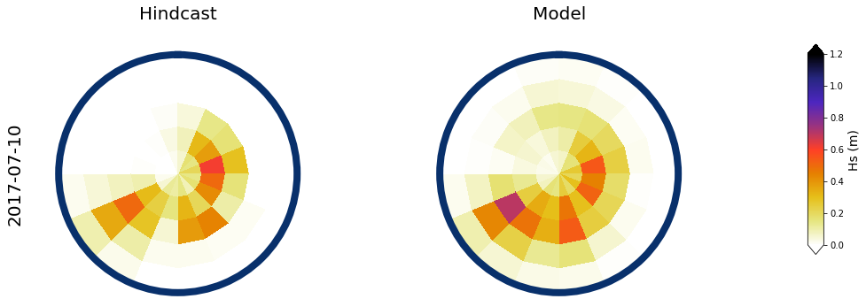
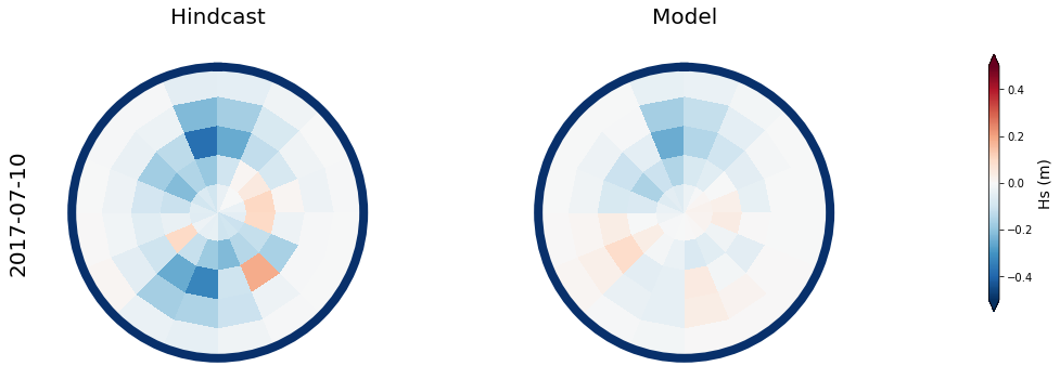
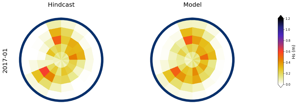
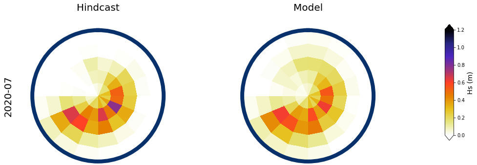
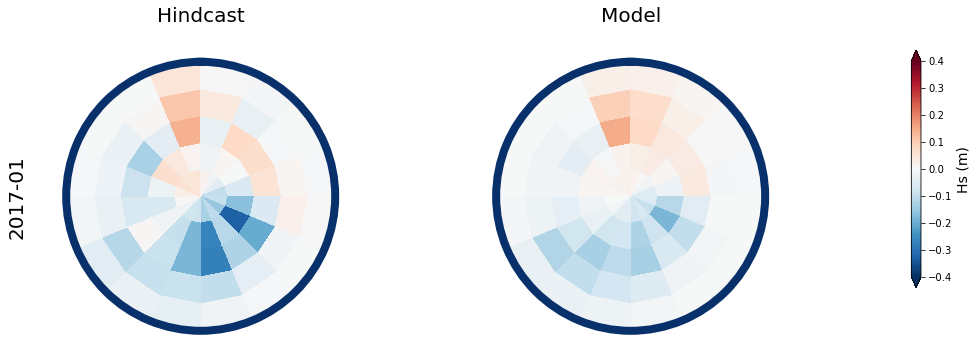
Also, the mean hindcast spectra and anomalies are shown below for comparison.
Mean model spectra is calculated as the sum of each cluster spectra multiplied by its probability of occurrence
# select a date to plot
day = '2017-07-10'

# slp for selected date
slp_d = slp_dy.sel(time = day)

# spectra hindcast for selected date
z = 4 * np.sqrt(sp_mod_daily.sel(time = day).h.values)

extent = (50, 290, -67, 65)

Plot_validation_spec(
    slp_d, spec_kma,
    extent = extent,
    real_spec = z,
    prob_min = 0, prob_max = 0.08,
    s_min = 990, s_max = 1030,
    lw = 4,
    pt = [184.84, -21.21],
    min_prob_clust = 0.02,
    title = day,
);


# daily mean spec
num_clus_pick = 49
perct_pick = []

# mean
Plot_daily_mean(
    slp_dy, sp_mod_daily,
    [day],
    spec_kma,
    num_clus_pick = num_clus_pick,
    perct_pick = perct_pick,
);


# anomaly (needs mean_spec)
mean_spec = 4 * np.sqrt(np.mean(sp_mod_daily.h.values, axis=0))

Plot_daily_mean(
    slp_dy, sp_mod_daily,
    [day],
    spec_kma,
    num_clus_pick = num_clus_pick,
    perct_pick = perct_pick,
    mean_spec = mean_spec,
    vmax=0.5, vmin=-0.5,
    cmap='RdBu_r',
);
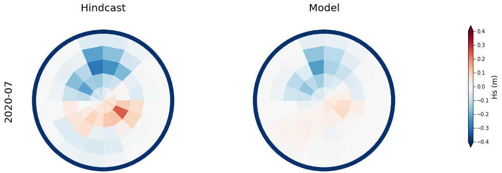
Results at the monthly scale#
For the purpose of the work, which is to develop a seasonal forecast, the results are aggregated to the monthly scale
The results for two months, one in January, and one in July are shown below
# resample slp and spectra to monthly data, using monthly means

slp_dy_m = slp_dy.resample(time = '1M', skipna = True).mean()

spec_mod_m = sp_mod_daily.resample(time = '1M', skipna = True).mean()
# select a month to plot
month = ['2017-01', '2020-07']

# SLP field and cluster probabilities
min_prob_clust = 0.005

# slp for selected month
slp_m = slp_dy_m.sel(time = month[0]).isel(time = 0)

# spectra hindcast for selected month
z = 4 * np.sqrt(spec_mod_m.sel(time=month[0]).isel(time=0).h.values)

a = Plot_validation_spec(
    slp_m, spec_kma,
    extent = extent,
    real_spec = z,
    prob_min = 0, prob_max=0.08,
    s_min = 990, s_max=1030,
    lw = 4,
    pt = [184.84, -21.21],
    min_prob_clust = 0.03,
    title = month,
);

# Monthly aggregated
num_clus_pick = 49
perct_pick = []

# mean
Plot_daily_mean(
    slp_dy_m, spec_mod_m,
    month,
    spec_kma,
    num_clus_pick = num_clus_pick,
    perct_pick = perct_pick,
);


# respect to the mean month spectra
mean_spec = 4 * np.sqrt(np.mean(spec_mod_m.h.values, axis=0))

# respect to the mean specific month
#mean_spec = 4 * np.sqrt(np.mean(spec_mod_m.isel(time=np.where(spec_mod_m.time.dt.month==slp_m.time.dt.month.values)[0]).h.values,axis=0))

# anomaly (needs mean_spec)
Plot_daily_mean(
    slp_dy_m, spec_mod_m,
    month,
    spec_kma,
    num_clus_pick = num_clus_pick,
    perct_pick = perct_pick,
    mean_spec = mean_spec,
    vmax = 0.4, vmin = -0.4,
    cmap = 'RdBu_r',
);
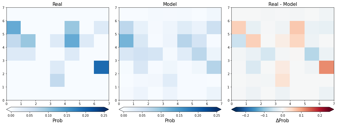
Compare cluster probabilities#
To compare the capabilities of the model on correctly reproducing the ocurrence probability of the different predicant clusters, we have compared the probabilities and calculated the relative entropy (RE) of real versus modelled probabilities
# spectral hindcast
sp_mod_daily = xr.open_dataset(p_sp_trans)

# select training time period
sp_mod_daily_fit = sp_mod_daily.sel(time = slice(time_train_1, time_train_2))

# load training PCA
ipca = pk.load(open(p_pca_spec_fit, 'rb'))
# organize spatial data into lines
m = np.full((len(sp_mod_daily.time), len(sp_mod_daily.dir_bins) * len(sp_mod_daily.t_bins)), 0.000001)

for ti in range(m.shape[0]):
    m[ti, :] = np.ravel(sp_mod_daily.h_t.isel(time = ti).values)

# calculate PCs
PCs_val = ipca.transform(m)
# load training kma
kma_fit = pk.load(open(p_kma_spec_model, 'rb'))[0]

# predict bmus
bmus_val = kma_fit.predict(PCs_val[:, :n_pcs_spec])

# sort bmus with kma order
kma_order = spec_kma.kma_order.values

sorted_bmus_val = np.zeros((len(bmus_val),),) * np.nan
for i in range(len(spec_kma.clusters)):
    posc = np.where(bmus_val == kma_order[i])
    sorted_bmus_val[posc] = i

# add sorted bmus to spectra dataset
sp_mod_daily['bmus'] = ('time', sorted_bmus_val.astype('int'))
Here, the comparison of real versus modelled probabilities is shown for a month
month = ['2017-03']

Plot_prob_comparison(sp_mod_daily, slp_dy_m, spec_kma, month);
RE = 0.5743748637250338
# calculate entropy
re_all = calculate_entropy(sp_mod_daily, slp_dy_m, spec_kma)
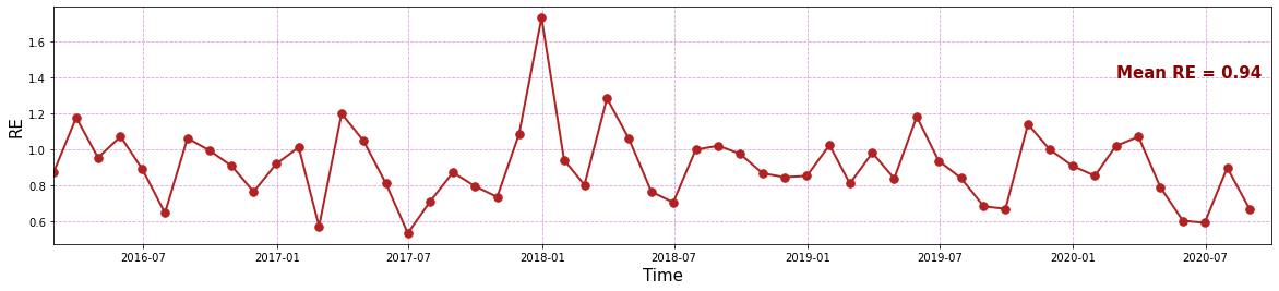
print('RE mean = ' + str(np.nanmean(re_all[1:])))
RE mean = 0.9411161735077451
Here, the RE for the validation period is shown
Plot_entropy(slp_dy_m, re_all);