Spectra conditioned to large scale predictors

In this section, we are going to find the link of the wave spectra with large scale climatic indices, as the Madden Julian Oscillation and El Niño 3.4, which characterized the ENSO variability of the area.

# common
import warnings
warnings.filterwarnings('ignore')
import os
import os.path as op
import sys

# pip
import numpy as np
import xarray as xr

# DEV: bluemath
sys.path.insert(0, op.join(op.abspath(''), '..', '..', '..', '..', '..'))

# bluemath modules 
from bluemath.binwaves.nino34 import n34_format

from bluemath.binwaves.plotting.nino34 import Plot_n34

from bluemath.plotting.mjo import Plot_mjo
from bluemath.plotting.spectra import Plot_spec_n34_mjo_month, Plot_spec_mjo, Plot_spec_n34, Plot_spec_months
from bluemath.plotting.spectra import Plot_spec_months_n34, Plot_spec_months_mjo, Plot_spec_months_mjo_n34sel

Database and site parameters

# database
p_data = r'/media/administrador/HD2/SamoaTonga/data'
site = 'Samoa'
p_site = op.join(p_data, site)

# Madden Julian Oscillation
p_mjo = op.join(p_data, 'mjo.nc')

# nino34 dataset
p_n34 = op.join(p_data, 'ninho34.txt')

# deliverable folder
p_deliv = op.join(p_site, 'd04_seasonal_forecast_swells')

# K-Means data
p_kma = op.join(p_deliv, 'kma')    

p_kma_spec_superpoint = op.join(p_kma, 'spec_KMA_classification.nc')   # classified superpoint

The Madden Julian Oscillation

The MJO is an eastward moving disturbance of clouds, rainfall, winds, and pressure that crosses the planet in the tropics and returns to its initial starting point in cycles of approximately 30 or 60 days. It is the dominant mode of atmospheric intraseasonal variability in the tropics.

The MJO consists of two phases: the enhanced rainfall and the the suppressed rainfall. They produce opposite changes in clouds and rainfall and this entire dipole propagates eastward. Strongest MJO activity often divides the planet into halves: one half within the enhanced convective phase and the other half in the suppressed convective phase.

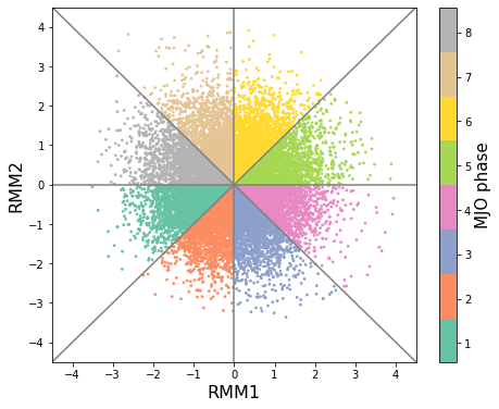
The MJO phases can be observed and represented through the RMM index, which is a combined cloudiness- and circulation-based index that has been frequently used for real-time prediction and definition of the MJO.

# Load suerpoint with KMeans classification data
sp_mod_daily = xr.open_dataset(p_kma_spec_superpoint)

# Load mjo
mjo = xr.open_dataset(p_mjo)

# Plot MJO
Plot_mjo(mjo);

El Niño 3.4

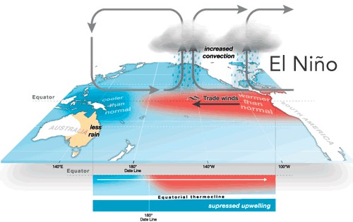
ENSO is one of the most important climate phenomena on Earth due to its ability to change the global atmospheric circulation; since it can lead to changes in sea-level pressures, sea-surface temperatures, precipitation and winds across the globe. ENSO describes the natural interannual variations in the ocean and atmosphere in the tropical Pacific. This interaction between the atmosphere and ocean is the source of a periodic variation between below-normal and above-normal sea surface temperatures and dry and wet conditions along the years. The tropical ocean affects the atmosphere above it and the atmosphere influences the ocean below it.

Typical behavior of the couple system of ocean and atmosphere during El Niño in the equatorial Pacific \(\href{http://www.bom.gov.au/watl/about-weather-and-climate/australian-climate-influences.shtml?bookmark=enso}{\text{(Australian Bureau of Meteorology)}}\):

# load ninho34 data
n34 = np.loadtxt(p_n34, skiprows=1, max_rows=74)
n34 = n34_format(n34, rolling_mean=True)

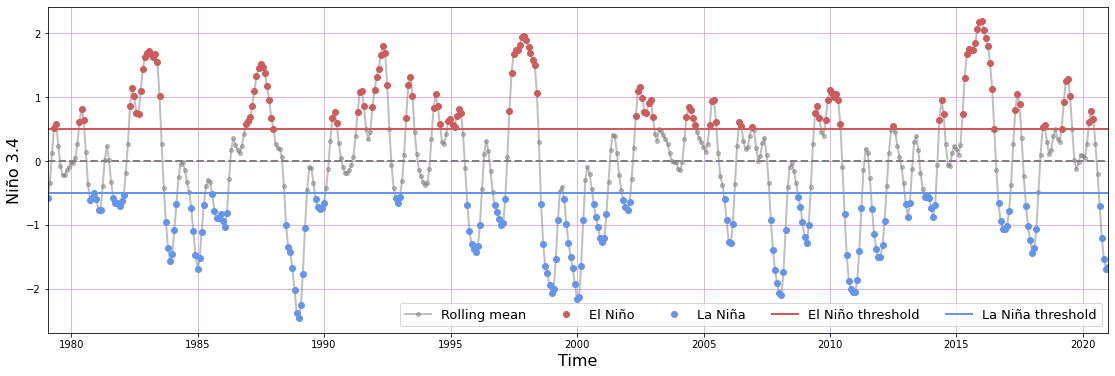
# plot ninho34 and thresholds
thr1 = 0.5   # over this value, years are classified as El Nino (1)
thr2 = -0.5  # under this value, years are classified as La Nina (3)
Plot_n34(n34, l1 = thr1, l2 = thr2, figsize=[19, 6]);

Spectra conditioned to:

Here we explore the mean values of the wave spectra conditioned to the different months of the year, the different phases of the MJO, the different classes of years based on El Niño 3.4 Index, and combinations of 2 or more of them

n34 = n34.resample(time='1D').interpolate("linear")

# find common dates for mjo, ninho34 and superpoint datasets
min_d = np.nanmax([mjo.time.values[0], n34.time.values[0], sp_mod_daily.time.values[0]])
max_d = np.nanmin([mjo.time.values[-1], n34.time.values[-1], sp_mod_daily.time.values[-1]])

n34 = n34.sel(time = slice(min_d, max_d))
mjo = mjo.sel(time = slice(min_d, max_d))
sp_mod_daily = sp_mod_daily.sel(time = slice(min_d, max_d))

# add mjo and ninho34 variables to superpoint classification
sp_mod_daily['mjo'] = ('time', mjo.phase.values)
sp_mod_daily['n34'] = ('time', n34.classification.values)

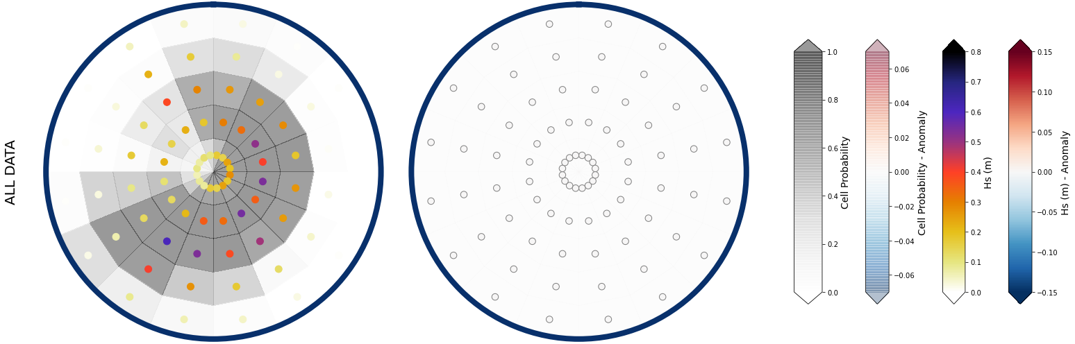
Mean Spectra and corresponding Annomaly
As we are representing the mean values, here there is no anomaly

n34_sel = []
mjo_sel = []
month = []

Plot_spec_n34_mjo_month(sp_mod_daily, n34_sel, mjo_sel, month, an_range=0.15, vmax_z1=0.8);

Number of data: 15161

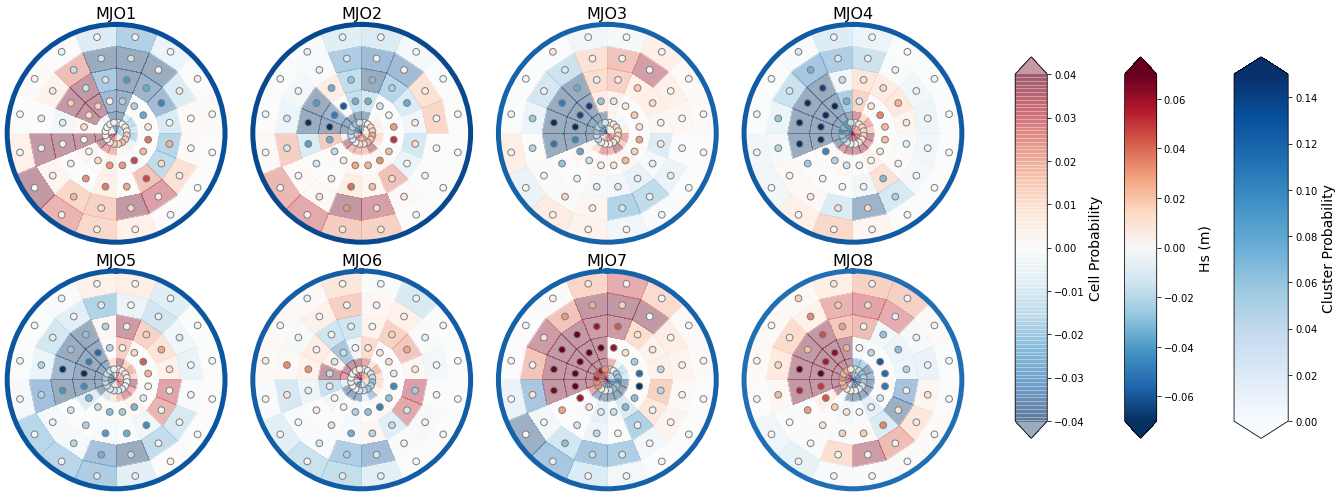
The MJO

Mean spectra conditioned to the 8 phases of the MJO and its anomaly from the mean
Phases 7 and 8, which are the most active phases in the area, have also the largest positive anomalies of waves coming from the west On the other hand, phases 3 and 4 have the largest negative anomalies of waves coming from the same directions. Also, phases 1 and 2, which are associated with the Indian and Africa area, are the phases with the greatest anomalies of large period swells arriving from south western directions.

Plot_spec_mjo(sp_mod_daily, vmax_z1=0.8);

Plot_spec_mjo(sp_mod_daily, annomaly=1, vmax_z1=0.07);

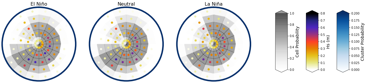
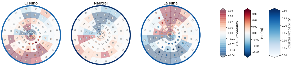
El Niño 3.4

Mean Spec conditioned to the 3 different clases of El Niño and its annomaly from the mean
During El Niño, a large anomaly of the number of large period swells arriving from the south, and an increase on the wave height of south eastern directions is observed As oposed, during La Niña, there is a negative anomaly both in the number and magnitude of Hs from the south, and a large anomaly from northern directions

Plot_spec_n34(sp_mod_daily, vmax_z1=0.8);

Plot_spec_n34(sp_mod_daily, annomaly=1, vmax_z1=0.07);

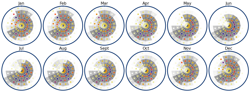
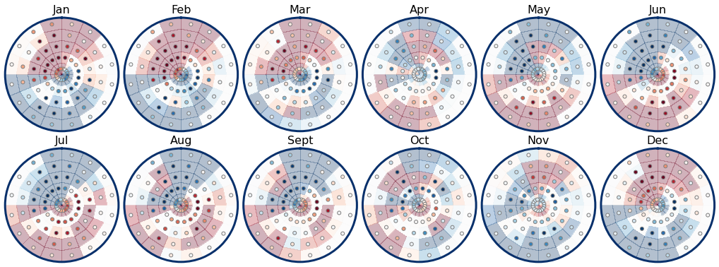
The month

Here, the seasonality of the wave spectra is shown
There is a clear pattern on the waves, where the boreal winter spectra is characterize by large and frequent wave systems from the north. On the other hand, the boreal summer is characterized by larger and more frequent waves coming from the south.

Note

From now on, there mean monthly values are used as the reference for calculating the anomalies.

Plot_spec_months(sp_mod_daily);

Plot_spec_months(sp_mod_daily, anomaly = 1);

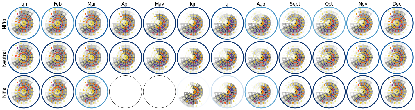
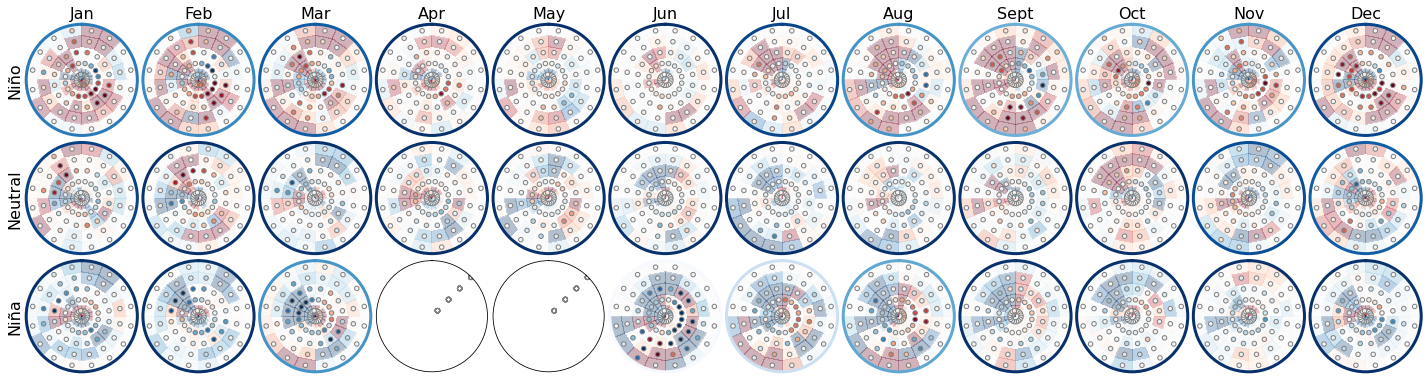
The month and El Niño3.4

Here, spectral information is conditioned both to the month and to the classification of El Niño 3.4 index, into El Niño, Neutral and La Niña

Plot_spec_months_n34(sp_mod_daily);

Plot_spec_months_n34(sp_mod_daily, anomaly=1, mean_month=1);

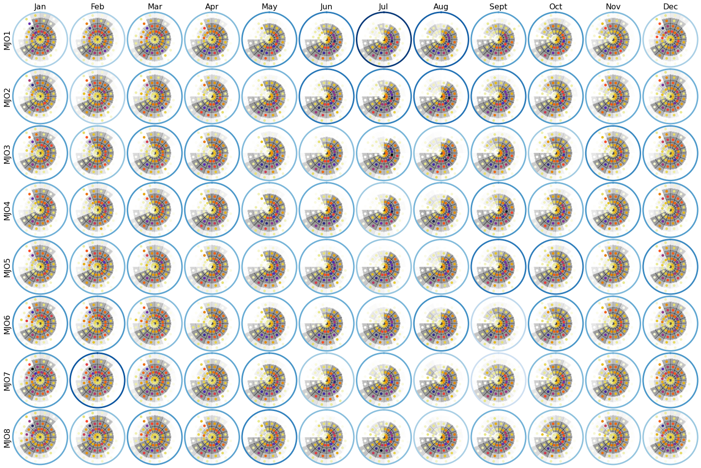
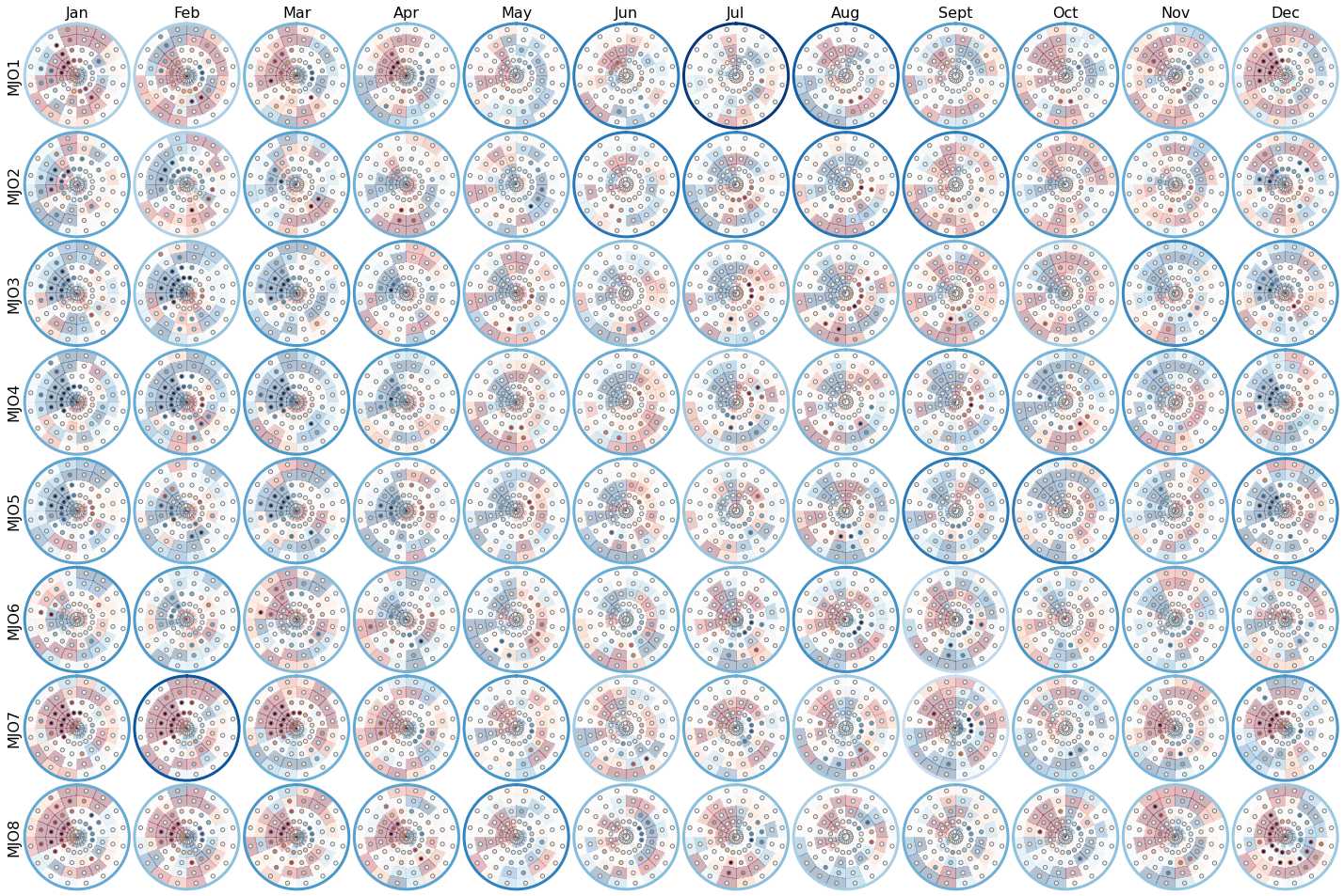
The month and the MJO

Here, spectral information is conditioned both to the month and to the 8 phases of the MJO

Plot_spec_months_mjo(sp_mod_daily, mean_month=1);

Plot_spec_months_mjo(sp_mod_daily, anomaly=1, mean_month=1);

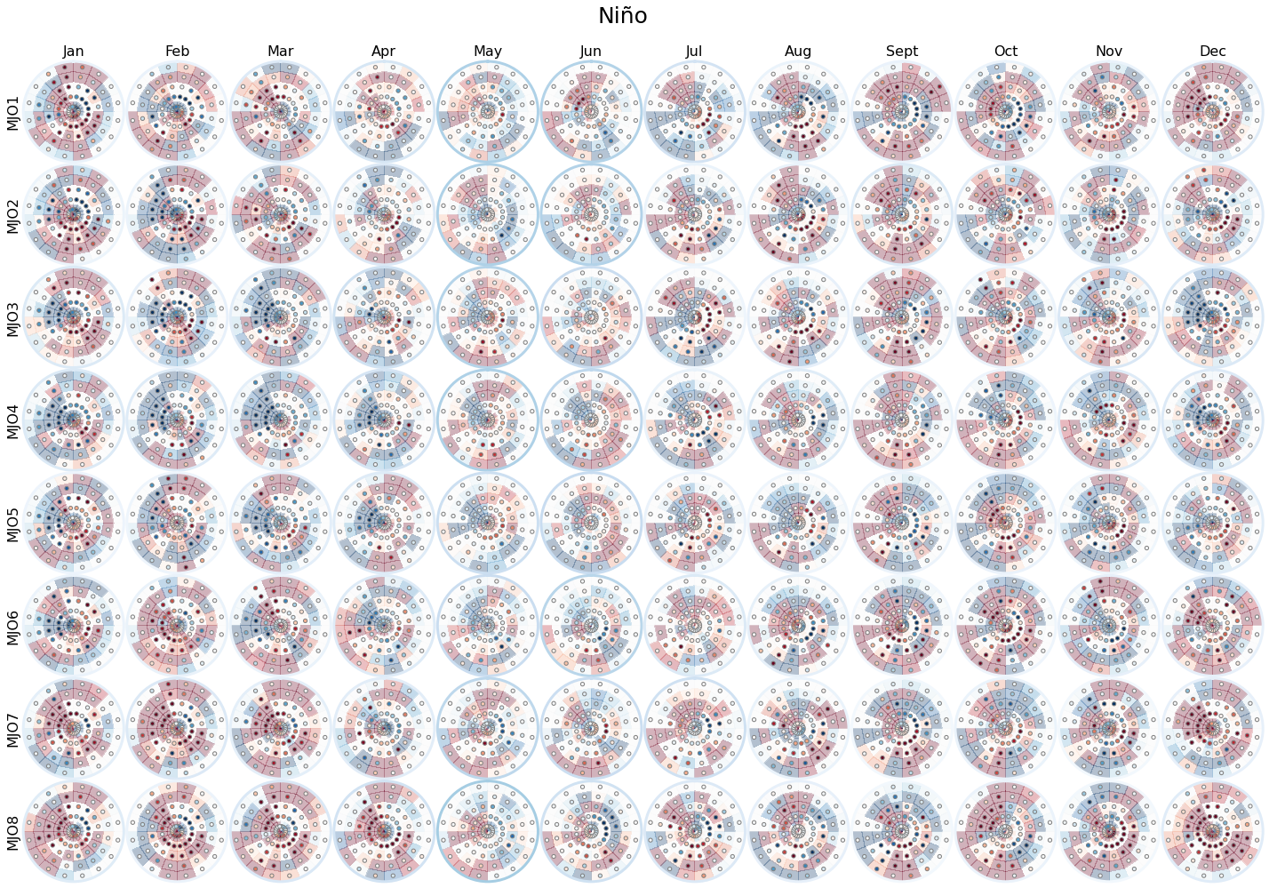
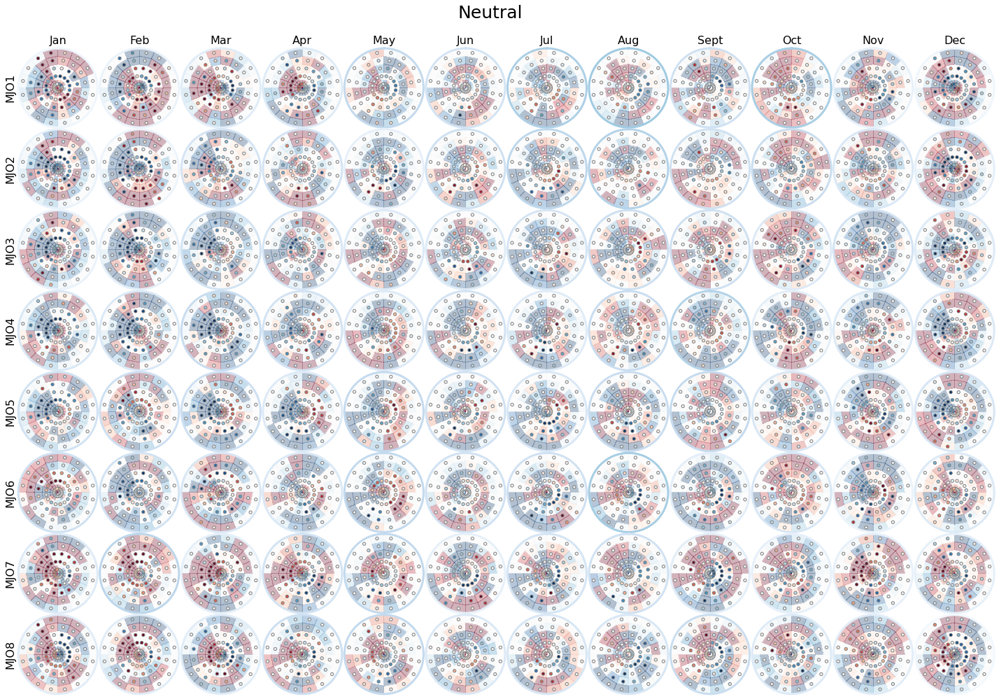
The month, the MJO and El Niño 3.4

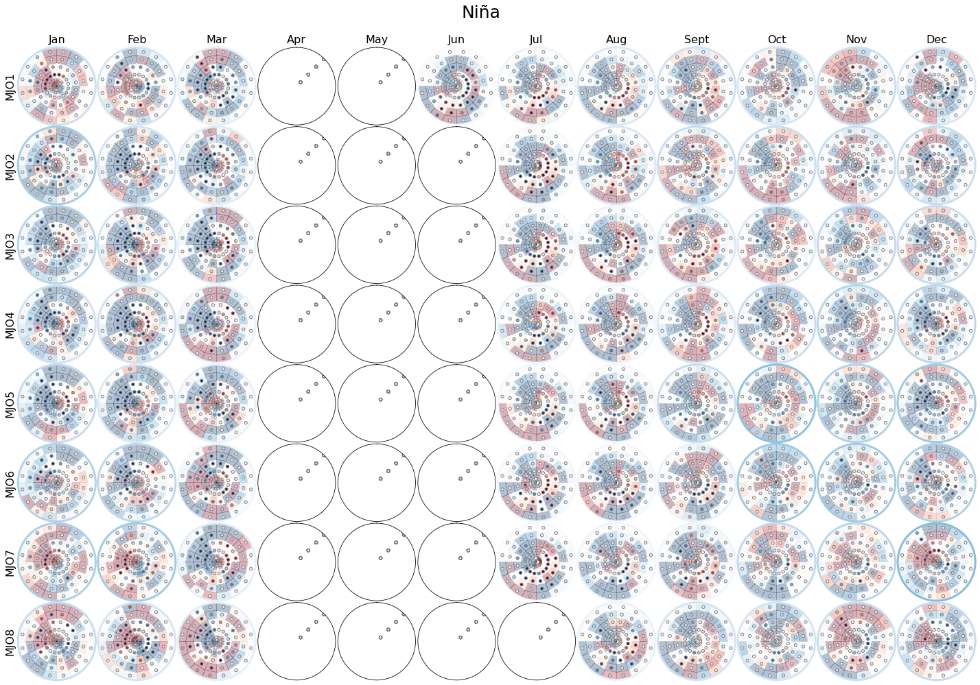
Here, the analysis is shown into 3 different figures, where the first one is conditioned to El Niño, the second one to Neutral years and the last one to La Niña

Plot_spec_months_mjo_n34sel(sp_mod_daily, n34_sel=1, anomaly=1, mean_month=1);

Plot_spec_months_mjo_n34sel(sp_mod_daily, n34_sel=2, anomaly=1, mean_month=1);

Plot_spec_months_mjo_n34sel(sp_mod_daily, n34_sel=3, anomaly=1, mean_month=1);

Example of Spectra conditioned to different number of predictors

Note

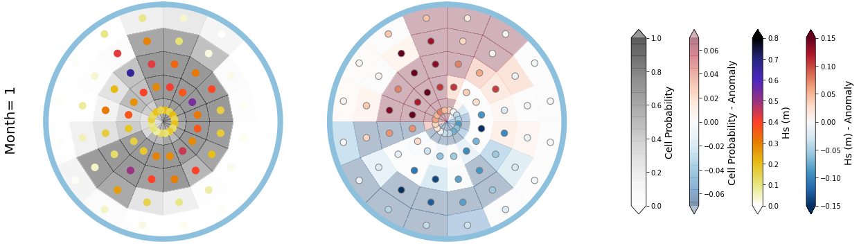
This example serves as an explanation on the influence of the different large scale climatic predictors on the wave spectra. For this purpose, we have selected a month (January) and incorporated the influence of El Niño 3.4 index and the MJO in 2 steps. This puts into evidence the influence of both predictors

Example of the mean spectra for January

Tip

If you are interested on extracting the data for any combination of month, MJO and El Niño, you can modify the different categories accordingly.
n34_sel can be set up to 1 (El Niño), 2 (Neutral) or 3 (La Niña).
mjo_sel can be set up from 1 to 8 and corresponds to the MJO phase.
month can be set up from 1 to 12 depending on the month of the year.

n34_sel = []  # 1:El Niño, 2:Neutral, 3:La Niña
mjo_sel = []
month = 1
mean_month = 0

Plot_spec_n34_mjo_month(sp_mod_daily, n34_sel, mjo_sel, month, an_range=0.15, mean_month=mean_month, figsize=[18,5]);

Number of data: 1272

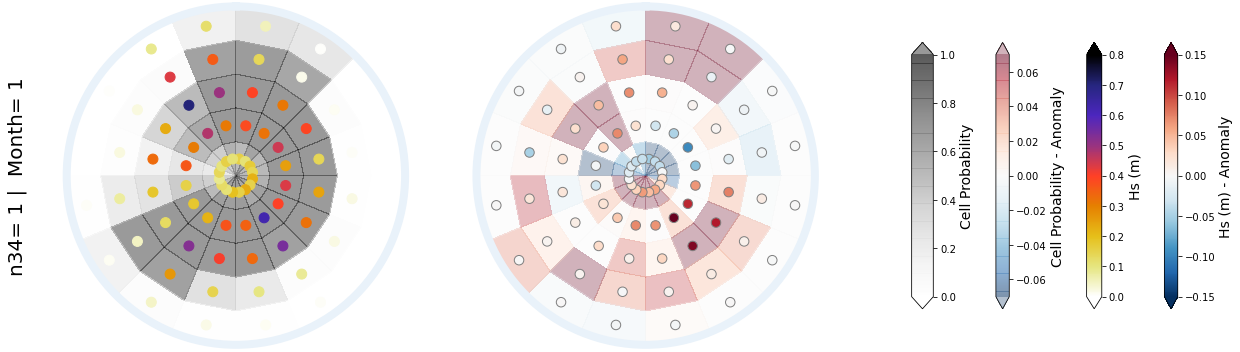
Example of the mean spectra for January conditioned to El Niño, and the annomaly with respect to the mean January

During El Niño, large positive Hs annomalies are observed specially for sea waves from the soth-east and an increase in the number of large swells from the north is observed

n34_sel = 1  # 1:El Niño, 2:Neutral, 3:La Niña
mjo_sel = []
month = 1
mean_month = 1

Plot_spec_n34_mjo_month(sp_mod_daily, n34_sel, mjo_sel, month, an_range=0.15, mean_month=mean_month, figsize=[18,5]);

Number of data: 217

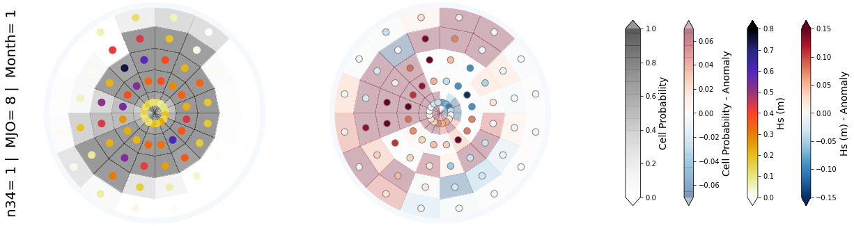
Example of the mean spectra for January conditioned to El Niño and a phase 8 of the MJO, and the annomaly with respect to the mean January

During phase 8 of the MJO, an active phase for this south Pacific area, an increase in the magnitude and frequency of wave systems approaching from the west is observed

n34_sel = 1  # 1:El Niño, 2:Neutral, 3:La Niña
mjo_sel = 8
month = 1
mean_month = 1

Plot_spec_n34_mjo_month(sp_mod_daily, n34_sel, mjo_sel, month, an_range=0.15, mean_month=mean_month, figsize=[18,5]);

Number of data: 36