.md .pdf

Contents

Velocity

The next magnitude that we can use to describe trajectories is the velocity. The velocity measures the change in the position with time. If an object occupies a position \(\vec{r}(t_1)\) in the initial time \(t=t_1\) and a position \(\vec{r}(t_1+\Delta t)\) after a short time \(\Delta t\) has passed since \(t_1\) (see Fig. 34) we can measure how much the object has moved using the vector,

(70)\[\Delta \vec{r} (t_1)= \vec{r}(t_1+\Delta t)-\vec{r}(t_1)\]

We will define velocity, \(\vec{v}\), as, precisely, the vector that measures this displacement as a linear function of the small time interval \(\Delta t\),

(71)\[\Delta \vec{r} (t_1)= \vec{r}(t_1+\Delta t)-\vec{r}(t_1) = \vec{v}\Delta t\]

The velocity, that corresponds with the fraction \(\Delta \vec{r}/\Delta t\) has dimensions of length divided by time so that its units in the international unit system is m/s.

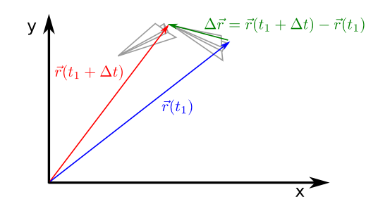
Fig. 34 Illustration of the change of position with time in the paper’s plane example. In the figure the plane takes a position \(\vec{r}(t_1)\) (blue vector) at the instant \(t=t_1\). When a time \(\Delta t\) has passed, the plane has moved to the point \(\vec{r}(t_1+\Delta t)\) (red vector). The vector \(\Delta \vec{r}\) (green) is the difference between these two vectors.

Mean velocity

If \(\Delta t\) is large, corresponding with typical times that we could measure with a watch or clock, we say that the velocity shown in Eq. (71) is called mean velocity.

(72)\[\vec{v}_m= \frac{\Delta \vec{r} (t_1)}{\Delta t} = \frac{\vec{r}(t_1+\Delta t)-\vec{r}(t_1)}{\Delta t}\]

When we use the mean velocity we consider that the object maintains a constant velocity, \(\vec{v}_m\), during the time interval \((t_1,t_1+\Delta t)\).

Instantaneous velocity

If \(\Delta t\) were very small, in the limit were it goes to zero and that, as a consequence, cannot be measured, we say that the velocity found in Eq. (71) is called instantaneous velocity (see Fig. 35).

(78)\[\vec{v}= \lim_{\Delta \to 0} \frac{\Delta t \vec{r} (t_1)}{\Delta t} = \lim_{\Delta t\to 0} \frac{\vec{r}(t_1+\Delta t)-\vec{r}(t_1)}{\Delta t}\]

The instantaneous velocity represents the real velocity that the object has at instant \(t=t_1\).

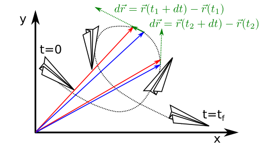
Fig. 35 As times passes the position vector changes adapting instantaneously its velocity.

Properties of the instantaneous velocity

In this section we want to study the direction of the velocity vector with respect to the trajectory. When the instantaneous velocity form is observed in detail,

(74)\[\vec{v}= \left(\frac{dx(t)}{dt},\frac{dy(t)}{dt},\frac{dz(t)}{dt} \right)\]

we see that its projection on the axes of the coordinate system correspond with the derivatives of the functions \(x(t)\), \(y(t)\) and \(z(t)\) that describe the trajectory. As it is well-known the geometric interpretation of the derivative is related to the slope of the tangent line to the curve described by the function. Given that the velocity vector is formed with the derivatives of \(x(t)\), \(y(t)\) and \(z(t)\) with respect to time, this vector is tangent to the three curves and, in general, to the trajectory.

This property can be graphically observed in Fig. 35 where it is possible to see that the vector \(\Delta \vec{r}\) gets closer to the tangent of the trajectorythe smaller \(\Delta t\) becomes (meaning when \(\Delta t \rightarrow dt\)).

Obtaining position from the velocity

Observing the equation for the position with the mean velocity (Eq. (71)) we can see that we can recover the position from the velocity simply by adding the areas of the rectangles of dimension \(\Delta t \times \vert v_m\vert\) (ver {numref}`mean_velocity_topos}),

(75)\[\Delta \vec{r} (t_1)= \vec{r}(t_1+\Delta t)-\vec{r}(t_1) = \vec{v}_m\Delta t \rightarrow \vec{r}(t_1+\Delta t)= \vec{r}(t_1)+\vec{v}_m\Delta t\]

Fig. 36 Mean velocity to position

Given the above, it seems clear that when \(\Delta t\) is very small (\(\Delta t \rightarrow 0\)), the sum of the areas will become an integral. This can be more clearly seen inverting equation (78) to find the position in terms of the instantanous velocity through time:

(78)\[\vec{v}= \frac{d\vec{r}}{dt} \rightarrow d\vec{r}=\vec{v}dt \rightarrow \int_{\vec{r}(t_0)}^{\vec{r}(t)}d\vec{r} = \int_{t_0}^{t} \vec{v}(t^\prime)dt^\prime \rightarrow \vec{r}(t)=\vec{r}(t_0) + \int_{t_0}^{t} \vec{v}(t^\prime)dt^\prime\]

Uniform motion

In the particular case of a uniform velocity En el caso particular de la velocidad uniforme,

(77)\[\vec{v}(t)=\vec{v} ~~\text{(constante)}\]

We can see that position is,

(78)\[\vec{r}(t)=\vec{r}(t_0) + \int_{t_0}^{t} \vec{v}dt^\prime =\vec{r}(t_0) + \vec{v} \int_{t_0}^{t} dt^\prime = \vec{r}(t_0) + \vec{v} (t-t_0)\]

as illustrated in Fig. 37.

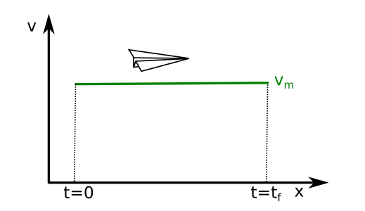
Fig. 37 Uniform velocity

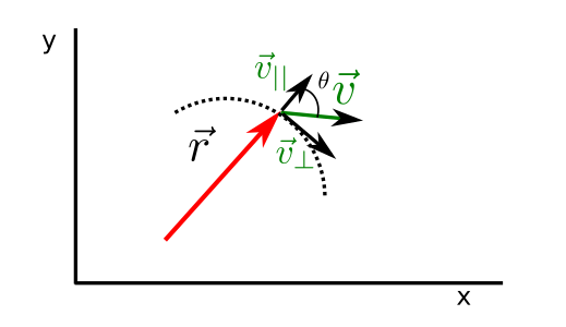
Fig. 38 Velocidad par perp

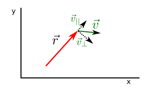
Fig. 39 Velocidad tan perp

Position and trajectory Acceleration