Circular movement¶

So far we have explored problems where the acceleration had a constant direction. One of the most important movement, the circular one requires that the acceleration changes direction so that the velocity vector accomodates to a closed, curved trajectory.

We will start by deducting the acceleration for a circular movement where the modulus of the velocity is kept constant to discuss the important emerging concepts like angular velocity. Then, we will move to the concepts of intrinsic components of the acceleration Intrinsic components of the acceleration and their relations with the angular acceleration.

Uniform circular motion¶

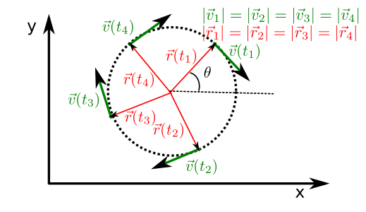
Fig. 44 During a circular motion the trajectory of the object is a circumference. As usual, the velocity vector is tangent to this circumference.¶

The uniform circular motion is one that verifies that,

the object moves along a circunference arc (circular) and
the modulus of its velocity is constant (uniform)

Looking at Fig. 44 we see that we can describe the position vector of a circular motion using polar coordinates, i.e.,

(97)¶\[\vec{r}=R\left(\cos(\theta(t))\vec{i}+\sin(\theta(t))\vec{j}\right)\]

Here, the system will travel around a circumference centered at the origin and with radius R if the rotation angle, \(\theta\), changes with time and R is kept constant. However, nothing here makes the movement uniform. In order to do so we need to calculate the velocity. Applying directly the definition of velocity we get,

(98)¶\[\vec{v}=\frac{d\vec{r}}{dt}=R\left(-\sin(\theta(t))\vec{i}+\cos(\theta(t))\vec{j}\right)\frac{d\theta}{dt}(t)\]

It is not difficult to see that this vector is perpendicular to the position vector and is tangent to the circumference (as expected for the velocity). Taking the modulus of the velocity we can now force it to take a constant value.

(99)¶\[\vert\vec{v}\vert=R\frac{d\theta}{dt}(t)=cte \Rightarrow \frac{d\theta}{dt}(t)=cte=\omega\]

Looking at the right-hand side of Eq. (98) we see that the constant \(\omega\) is the variation of the rotation angle with time and, for that reason, is usually called angular velocity.

Focusing now on the left-hand side of Eq. (98) we can observe an important, general relationship. The modulus of the (linear) velocity is the angular velocity times the radius of the trajectory,

(100)¶\[\vert\vec{v}\vert=R\frac{d\theta}{dt}=R\omega\]

Thus,

Acceleration in the uniform circular motion¶

If we now assume that \(\omega\) and \(R\) are constants in time, then the modulus of the velocity is constant too. Using the definition of angular velocity we can now find the explicit formula for the variation of the angle \(\theta\) in time,

(101)¶\[\frac{d\theta}{dt}(t)=\omega \Rightarrow \theta_f - \theta_i = \int_{t_i}^{t_f}d\theta = \int_{t_i}^{t_f}\omega dt = \omega (t_f - t_i) \Rightarrow \theta(t)=\theta_i+\omega (t - t_i)\]

Note that this formula is completely analogous to the uniform motion (78) when replacing the position by the rotation angle and the linear velocity by the angular velocity. Using this expression in our circular trajectory we can now obtain the acceleration by deriving the velocity with respect to time,

(109)¶\[\begin{split}\vec{a}=\frac{d\vec{v}}{dt}&=R\omega^2\left(-\cos(\theta_0+\omega t)\vec{i}-\sin(\theta_0+\omega t)\vec{j}\right)\\ &=-R\omega^2\frac{\vec{r}}{R}=-R\omega^2\vec{u}_\rho\end{split}\]

Thus, we see that the acceleration in a uniform circular motion is always,

radial as it is proportional to the polar unitary vector in this direction \(\vec{u}_\rho\)
directed to the center of the circumference as can be seen by the negative sign in Eq. (109)

Moreover, we can see that it proportional to the radius and the angular velocity squared.

Intrinsic components of the acceleration¶

At this point, it is convenient to define a general decomposition of the acceleration that provides much information during the movement. In order to decomponse the acceleration we will create a set of axes that changes during the trajectory,

one of the axes points along the direction of the velocity and it is, as a consequence, tangent to the trajectory.
the other axis points is simply perpendicular to the previous one and contains all the normal contribution to the acceleration.

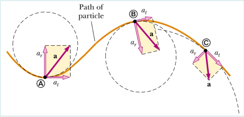
../../_images/componentes_aceleracion.png

Fig. 45 The acceleration is decomposed, at each point of the trajectory, into parallel (tangent) and perpendicular (normal) components.¶

The component of the acceleration that runs along the direction of the velocity is called tangential acceleration, \(\vec{a}_t\), while the one pointing in the perpendicular direction is called normal acceleration, \(\vec{a}_r\). They are illustrated in Fig. 45 and together the add up to the full acceleration.

(103)¶\[\vec{a}=\vec{a}_r+\vec{a}_t\]

Given that the tangential acceleration points in the direction of the velocity using Eq.(88) we can immediately see that the direction of the velocity does not change with it but its modulus does,

(104)¶\[\vert\vec{a}_t\vert=\frac{d\vert\vec{v}\vert}{dt}\]

Thus, the tangential acceleration is the sole responsible for the change in the modulus of the velocity.

On the other hand, the normal or centripetal acceleration is the only one that appears in the uniform circular motion (see above),

(105)¶\[\vert\vec{a}_r\vert = R\omega^2=\frac{\vert\vec{v}\vert^2}{R}\]

and is the sole responsible for the change in the direction of the velocity vector. As seen in Eq. (105) it is proportional to the square of the linear velocity and inversely proportional to the radius of the trajectory.

Angular acceleration¶

In a similar way that we defined the linear acceleration we can now define the angular acceleration, \(\alpha\), as

(106)¶\[\alpha=\frac{d\omega}{dt}\]

If we assume that the radius of the trajectory is constant we can find that the change of the modulus of the velocity is,

(107)¶\[\frac{d}{dt} \vert\vec{v}\vert=\frac{d}{dt} R\omega=R\frac{d\omega}{dt}=R\alpha\]

Given that this value is the tangential acceleration we find that,

(108)¶\[a_t=\frac{d\vert\vec{v}\vert}{dt} =R\alpha\]

Thus, in a circular trajectory, the tangential acceleration is proportional to the angular acceleration.

Angular velocity and acceleration vectors¶

In many cases we will follow the trajectory of an object in three dimensions, in those cases it is useful to define the angular velocity and accelerations as vectors.

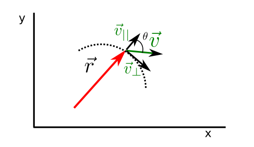
Fig. 46 movimiento circular¶

Looking at Fig. 46 we can define the velocity corresponding to the circular motion as that perpendicular to the radius of the trajectory. Using this component of the velocity and the definition of the angular velocity we find,

(109)¶\[\omega=\frac{v_\perp}{r}=\frac{\vert \vec{v}\vert \sin \theta}{r}\rightarrow\vec{\omega}=\frac{\vec{r}\times\vec{v}}{\vert\vec{r}\vert^2}\]

where, in the last step we inducted the formula from the modulus of the cross product. In a similar way, we can find the linear velocity from the angular velocity vector as,

(110)¶\[\vec{v}=\vec{\omega}\times\vec{r} \]

Armed with this definition we can now derive the expression in time and identify the terms in the resulting expression with the intrinsic components of the acceleration,

(111)¶\[\vec{a}=\frac{d\vec{v}}{dt}=\frac{d\vec{\omega}}{dt}\times\vec{r}+\omega\times\frac{d\vec{r}}{dt}\]

From Eq. (111) we see that the second term on the right-hand side is perpendicular to the velocity and so is the centripetal acceleration,

(112)¶\[\vec{a}_c=\vec{\omega}\times\frac{d\vec{r}}{dt}\]

while the other term that is proportional to the angular acceleration is the tangential acceleration,

(113)¶\[\vec{a}_t=\frac{d\vec{\omega}}{dt}\times\vec{r}=\vec{\alpha}\times\vec{r}\]

Física General