.md .pdf

Contents

Acceleration

Similarly to the way in which velocity was introduced as the change of position with time, in this section we will define acceleration as the change of velocity with time. It is worthwhile to notice that this procedure can be extended and we could then come to think about how acceleration changes with time and start defining another magnitude (called jerk or jolt, sobreaceleración/tirón in Spanish) to then think about how this jerk changes in time in a never-ending cycle. As we will see over the next chapter, devoted to dynamics, acceleration is a special magnitude as it is directly connected to forces and the origin of movement.

When we observe an object in movement as, for example, the paper plane that we used in previous sections (see Fig. 40), we will often observe that the velocity is not constant but that it changes both in modulus (the plane becomes slower as it climbs and moves faster as it descends) and in direction direction (when it performs a loop).

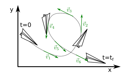
Fig. 40 Paper plane is accelerated.

The change in the velocity vector with time is known as acceleration. As can be expected this magnitude has dimensions of length over time squared ad in the international unit system is measured in \(m/s^2\).

Mean acceleration

In the same way that we acted with the velocity, if we observe the change of velocity with the help of a chronometer with a time resolution \(\Delta t\), meaning, using a time scale large enough to be measured, acceleration takes the value,

(79)\[\vec{a}_m= \frac{\Delta \vec{v} }{\Delta t} = \frac{\vec{v}_f-\vec{v}_i}{t_f-t_i}\]

where \(t_f\) and \(t_i\) are the final and initial times of the measurement and \(\vec{v}_f\) and \(\vec{v}_i\) are the corresponding velocities at these times.

As in the case of mean velocity, the use of mean acceleration implies that we are considering that the acceleration is constant over time intervals of length \(\Delta t\).

Instantaneous acceleration

If we now consider that we can measure the acceleration in very small time intervals (\(\Delta t \rightarrow 0\)) we could define acceleration with full precision at every instant,

(80)\[\vec{a}= \lim_{\Delta t\rightarrow 0} \frac{\Delta \vec{v} }{\Delta t} =\lim_{\Delta t\rightarrow 0} \frac{\vec{v}(t+\Delta t)-\vec{v}(t)}{\Delta t}\]

Position and velocity from acceleration

In order to find the velocity we will use the definition of acceleration to find:

(81)\[\frac{d\vec{v}}{dt}=\vec{a} \Rightarrow d\vec{v}=\vec{a}dt\]

We can now integrate Eq. (81) between the initial time, \(t_i\), and the final time, \(t_f\):

(82)\[\int_{t_i}^{t_f}d\vec{v}=\vec{v}\vert_{t_i}^{t_f}=\vec{v}_f-\vec{v}_i=\int_{t_i}^{t_f}\vec{a}(t)dt\]

In order to find the position we will take the initial time to be \(t_i=t_0\) and we let the final time to be variable \(t_f=t\), then:

(83)\[\vec{v}_f=\vec{v}(t)=\vec{v}_0+\int_{t_0}^{t}\vec{a}(t^\prime)dt^\prime\]

As in usual integration in this process we find an integration constant that, in this case, corresponds with the velocity at the initial time (\(t_0\)) and that we denote \(\vec{v}_0\). Once that Eq. (83) has been found we can integrate a second time with respect to time to find the position:

(84)\[\frac{d\vec{r}}{dt}=\vec{v} \Rightarrow d\vec{r}=\vec{v}dt\rightarrow \int_{t_0}^{t}d\vec{r}=\int_{t_0}^{t}\vec{v}(t^\prime)dt^\prime\]

Integrating on the left-hand side and substituting by the expression of the velocity, Eq. (83), we find,

(85)\[\begin{split}\vec{r}(t)=\vec{r}_0+\int_{t_0}^{t}\vec{v}(t^\prime)dt^\prime \Rightarrow \vec{r}(t)&=\vec{r}_0+\int_{t_0}^{t}\left(\vec{v}_0+\int_{t_0}^{t^\prime}\vec{a}(t^{\prime\prime})dt^{\prime\prime}\right)dt^\prime\\ &=\vec{r}_0+\vec{v}_0\int_{t_0}^{t}dt^\prime+\int_{t_0}^{t}\int_{t_0}^{t^\prime}\vec{a}(t^{\prime\prime})dt^{\prime\prime} dt^\prime \\ &=\vec{r}_0+\vec{v}_0 (t-t_0)+\int_{t_0}^{t}\int_{t_0}^{t^\prime}\vec{a}(t^{\prime\prime})dt^{\prime\prime} dt^\prime\end{split}\]

where, again, we find an integration constant that, in this case, we can interpret as the initial position, \(\vec{r}_0\), that the object had at the initial time (\(t=t_0\)).

Uniformly accelerated movement

The goal of this section is finding the velocity and position of an object that has a constant acceleration in time. We say that the movement of this object is uniformly accelerated. In order to do so we will follow the previous section with the simplification that we will now consider the acceleration vector constant leading to trivial integrals. Using the definition of acceleration we find:

(86)\[\frac{d\vec{v}}{dt}=\vec{a} \Rightarrow d\vec{v}=\vec{a}dt\]

We can now integrate Eq. (86) between the initial time, \(t_i\), and the final time, \(t_f\):

(87)\[\begin{split}\int_{t_i}^{t_f}d\vec{v}=\vec{v}\vert_{t_i}^{t_f}=\vec{v}_f-\vec{v}_i=\int_{t_i}^{t_f}\vec{a}dt=\vec{a}\int_{t_i}^{t_f}dt=\vec{a}(t_f-t_i)\\ \vec{v}_f-\vec{v}_i=\vec{a}(t_f-t_i)\Rightarrow\vec{v}_f=\vec{v}_i+\vec{a}(t_f-t_i)\end{split}\]

Now we can generalize that the initial time is \(t_i=t_0\) and we let the final time to be variable \(t_f=t\) entonces:

(88)\[\vec{v}_f=\vec{v}(t)=\vec{v}_0+\vec{a}t\]

As in usual integration in this process we find an integration constant that, in this case, corresponds with the velocity at the initial time (\(t_0\)) and that we denote \(\vec{v}_0\). Once that Eq. (88) has been found we can integrate a second time with respect to time to find the position:

(89)\[\begin{split}\vec{r}_f=\vec{r}_i+\int_{t_i}^{t_f}\vec{v}(t)dt \Rightarrow \vec{r}(t)&=\vec{r}_0+\int_{t_i=0}^{t_f=t}\left(\vec{v}_0+\vec{a}t^\prime\right)dt^\prime\\ &=\vec{r}_0+\vec{v}_0\int_{t_i=0}^{t_f=t}dt^\prime+\vec{a}\int_{t_i=0}^{t_f=t}t^\prime dt^\prime \\ &=\vec{r}_0+\vec{v}_0 t +\frac{1}{2} \vec{a} t^2\end{split}\]

where, again, we find an integration constant that, in this case, we can interpret as the initial position, \(\vec{r}_0\), that the object had at the initial time (\(t=t_0\)).

Mean rectilinear accelerated movement

Considering the results in the previous section we can graphically represent by the result considering that the moving object has an average acceleration, \(a_i\) is applied over intervals of time \(\Delta t_i\) (see Fig. 41). In that case the total velocity is the area underneath the function \(a(t)\) can be obtained by adding the area of the rectangles \(a_i \times \Delta t_i\).

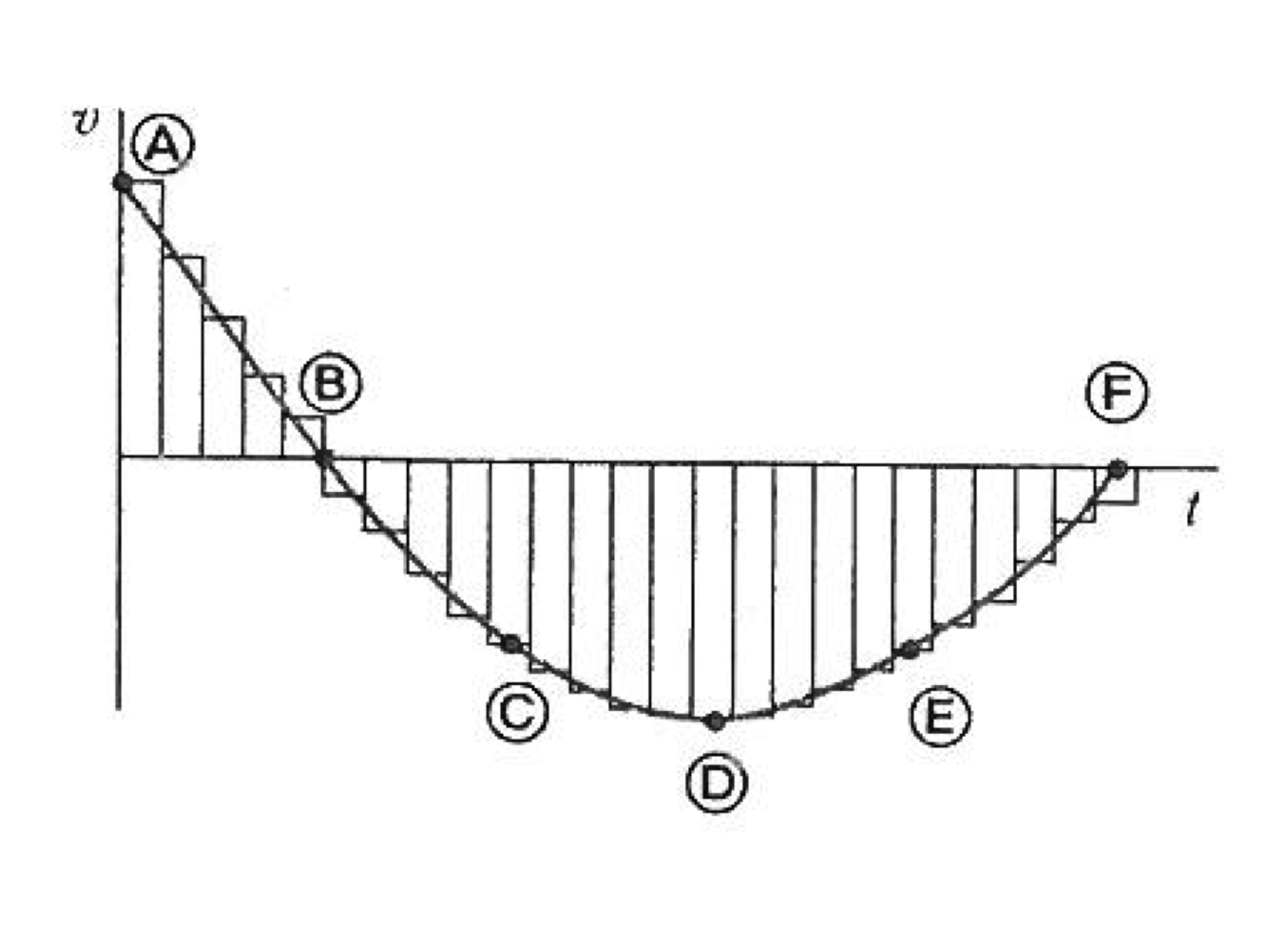
Fig. 41 The acceleration can be obtain by adding the areas of small rectangles,

Problems and solved examples

Velocity Examples of movement