HyBeat metamodel: selection of cases, generating a library of pre-run cases and PCA analysis

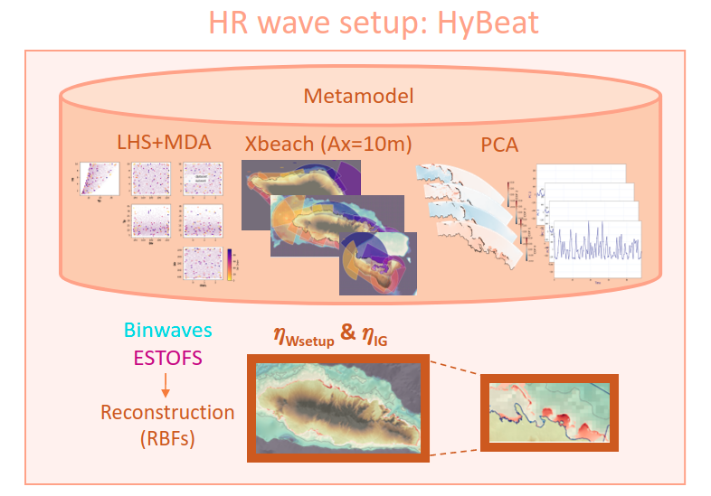
HyBeat is a metamodel based on datamining techniques and a reduced number of 2D hydrodynaimc model Xbeach (Roelvink et al., 2015) numierical simulations, that allows to obtain the mean setup and the infragravity wave at a very high resolution (~ 5-20m) at the coast.

These are the steps followed in the HyBeat methodology:

• Selection of 100 design cases based on selected parameters (Hs,Tp, θ, 𝜂) using Latin Hybercube Sampling (LHS) algorithm and Maximum Dissimilarity Algorithm (MDA) selection technique
  

• Numerically run the 100 design cases per each computational grid with the 2D model Xbeach at a spatial resolution of 5 to 20 meters
  

• Post process the 100 simulations per computational domain by means of Principal Component Analysis (PCA)
  

HyBeat

In this notebook we are going to focus on showing significant intermediate results of HyBeat metamodel to be able to reconstruct any given event

# common
import os
import sys
import warnings
warnings.filterwarnings('ignore')

# pip
from scipy.stats import qmc
import pandas as pd
import numpy as np
from sklearn.cluster import KMeans


# bluemath 
sys.path.insert(0, os.path.join(os.path.abspath(''),  '..'))
from Codes.LHS import *
from Codes.mda import MaxDiss_Simplified_NoThreshold
from Codes_v3.Codes.plots import *

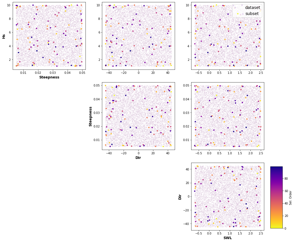
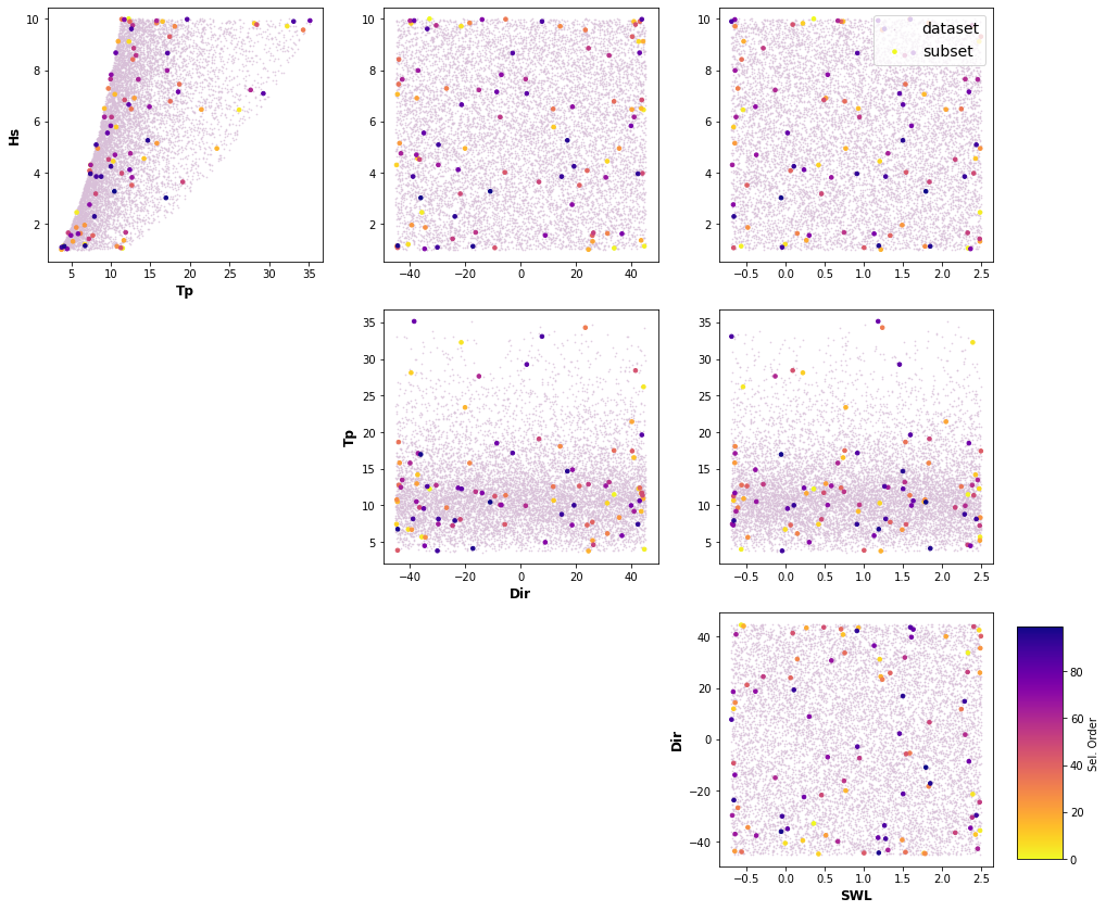
LHS + MDA

A selection of cases based on selected parameters (Hs,Tp, θ, 𝜂) and its ranges is done through Latin Hypercube Sampling algorithm (LHS, McKay et al., 1979, Sheikholeslami and Razavi, 2017) and a selection algorithm, Maximum Dissimilarity Algorithm (MDA, Camus et al., 2011a). LHS cuts each dimension space into n (10,000) sections, where n is the number of sampling points, and only one combination in each section is kept. It produces samples that reflect the true underlying distribution, and it tends to require much smaller sample sizes than simple random sampling. Then Hs,Tp, θ and 𝜂 variables are chosen to apply MDA, with the aim of selecting a representative subset of 100 cases which best captures the variability of the space.

HyBeat

The following intermediate results are for Apia domain in Upolu island

#Ocean parameters
n_dims = 4 #Number of dimensions
name_dims=['Hs', 'Steepness', 'Dir', 'SWL']
lower_bounds = [1, 0.005, -45, -0.7] 
upper_bounds = [10, 0.05, 45, 2.5]
n_samples=10000 #Number of combinations to extract from LHS

#LHS params and selection
sampler = qmc.LatinHypercube(d=n_dims,seed=0)
dataset = sampler.random(n=n_samples)
dataset = qmc.scale(dataset, lower_bounds, upper_bounds)
dataset_pd = pd.DataFrame(dataset, columns=name_dims).to_xarray()
dataset_pd['Tp'] = (('index'), np.sqrt((dataset_pd.Hs.values*2*np.pi)/(9.81*dataset_pd.Steepness.values)))

#MDA selection
n_subset = 100 #Subset for MDA
ix_scalar = [0,1,3]
ix_directional = [2]

subset_mda = MaxDiss_Simplified_NoThreshold(dataset, n_subset, ix_scalar, ix_directional)
df = pd.DataFrame(subset_mda, columns=name_dims).to_xarray()
df['Tp'] = (('index'), np.sqrt((df.Hs.values*2*np.pi)/(9.81*df.Steepness.values)))

MaxDiss dataset: 10000 --> 100

   MDA centroids: 100/100

n=100
Plot_MDA_Data(pd.DataFrame(dataset), pd.DataFrame(subset_mda[:n,:]), d_lab=name_dims, figsize=[15,12])

dataset_plot = np.vstack([dataset_pd['Hs'].values, dataset_pd['Tp'].values, dataset_pd['Dir'].values,dataset_pd['SWL'].values]).T
mda_plot = np.vstack([df['Hs'].values, df['Tp'].values, df['Dir'].values,df['SWL'].values]).T
name_plot=['Hs', 'Tp', 'Dir', 'SWL']

Plot_MDA_Data(pd.DataFrame(dataset_plot), pd.DataFrame(mda_plot[:n,:]), d_lab=name_plot, figsize=[15,12])

Library of Xbeach pre-run cases

A set of computational grids are carefully design according to the HR topo-bathymetry data (5 m) so that the wave setup results along the entire coastline of the islands is well defined without instabilities due to lateral boundary conditions. The following figure shows the domain of each computational grid for Upolu island, as well as the overlapping areas between them. These computational grids are generated using Delft3D (https://oss.deltares.nl/web/delft3d) meshing tools RFGRID and QUICKIN, which enables the generation of rectilinear and curvilinear grids from higher (~ 80m) to lower resolution (~ 5-20m) near the coast. Finally, each model run simulates in surfbeat mode a one-hour event according the 100 design cases, which Hydraulic Boundary Conditions (HBCs) are defined by a parametric Jownsap spectra and a constant water level (Hs,Tp, θ, 𝜂).

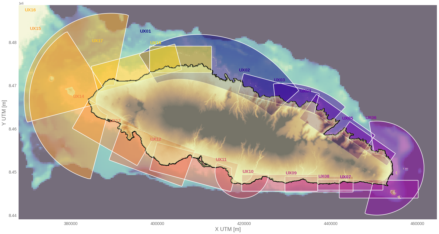
HyBeat

The following intermediate results are for Apia domain in Upolu island

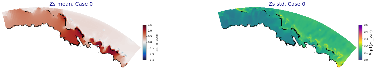
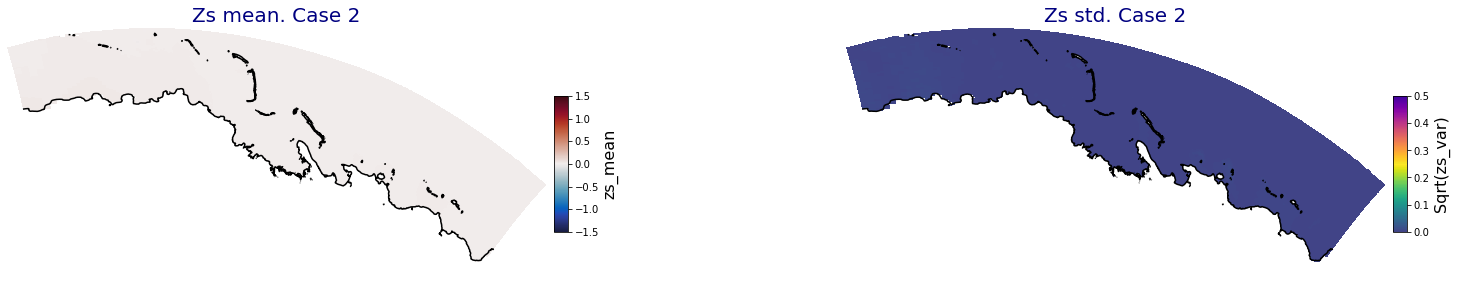
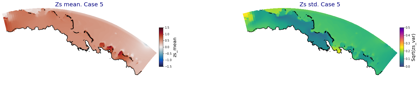
p_results = '/media/administrador/HD/SamoaTonga/xbeach/Cluster/Results/Postprocess_results/Upolu/PCA_results/UX01'
C_R_zs_mean = xr.open_dataset(os.path.join(p_results, 'PCA_zs_mean_ncases_100.nc'))
C_R_zs_var = xr.open_dataset(os.path.join(p_results, 'PCA_zs_var_ncases_100.nc'))

ncases = len(C_R_zs_mean.case)
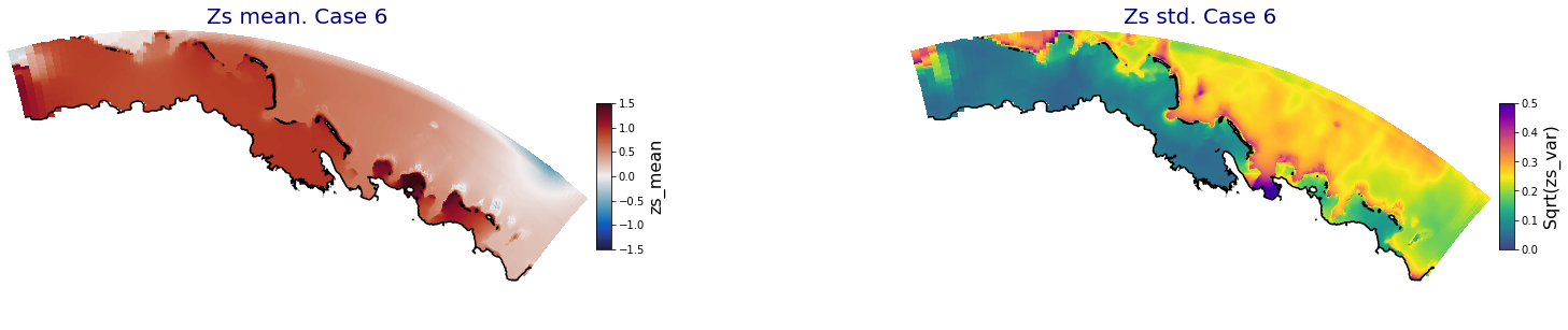
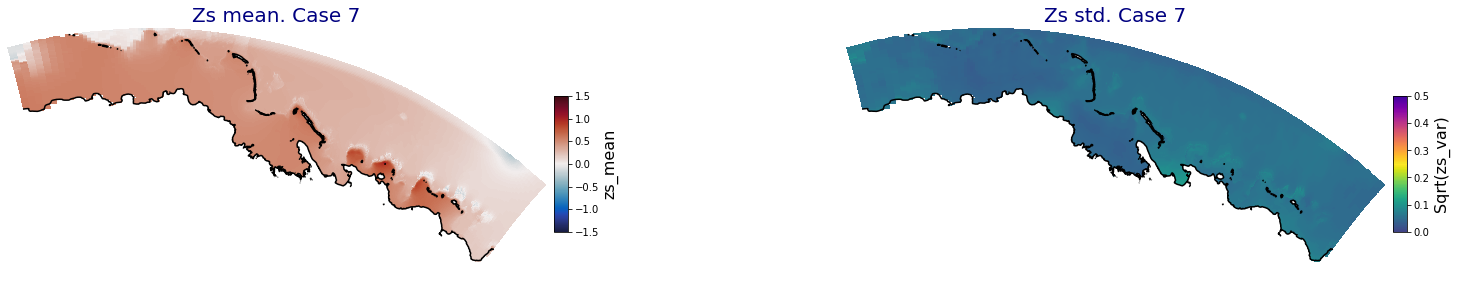
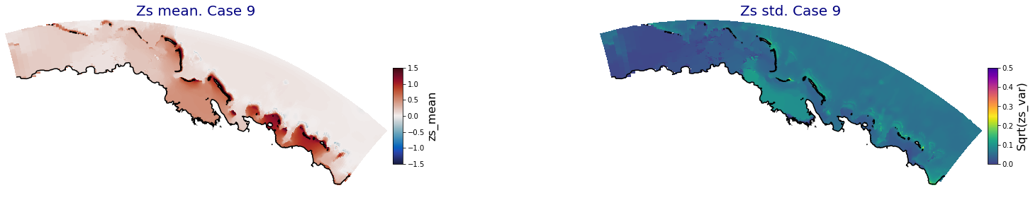
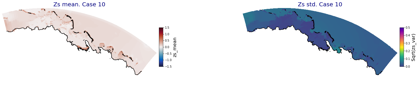
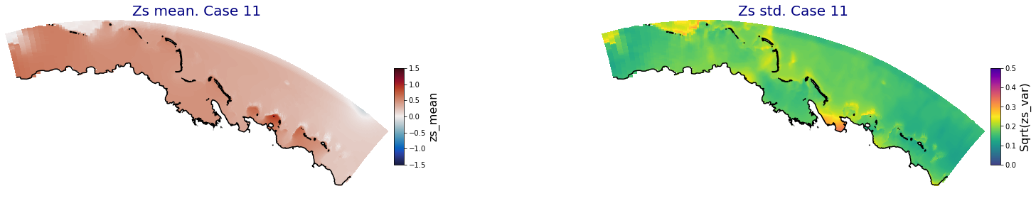
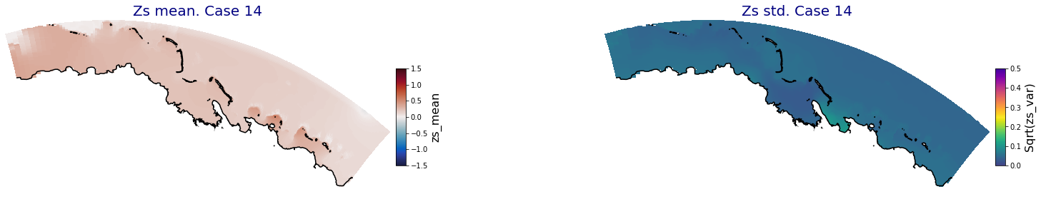
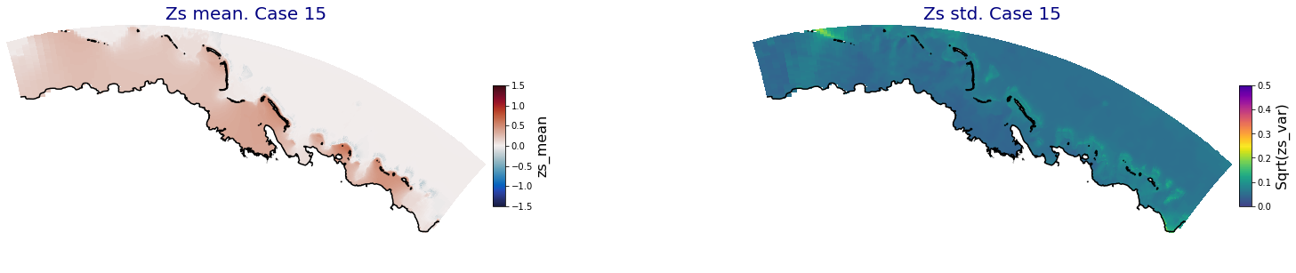
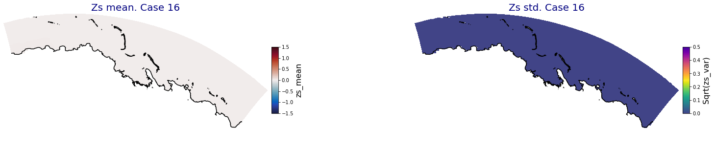
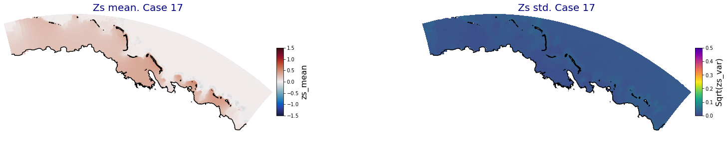
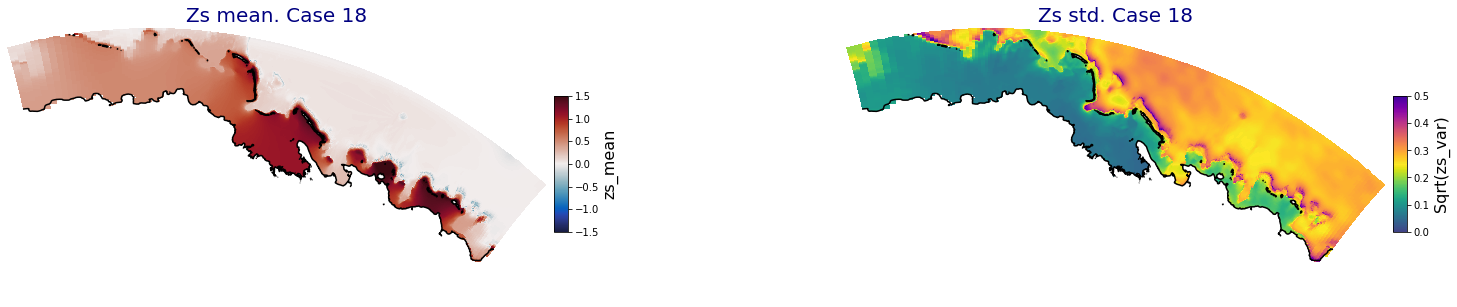
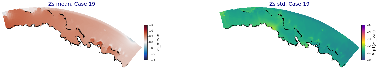
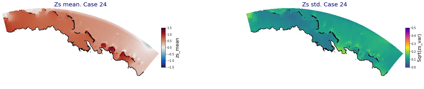
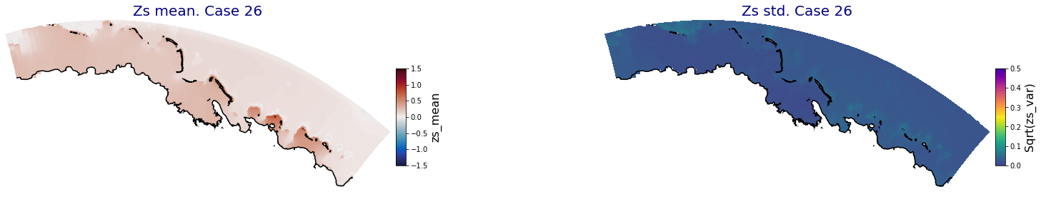
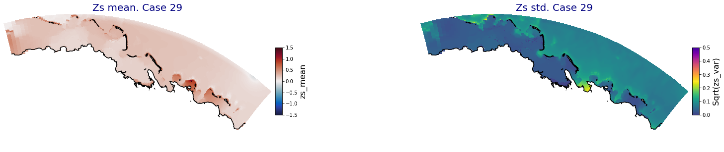
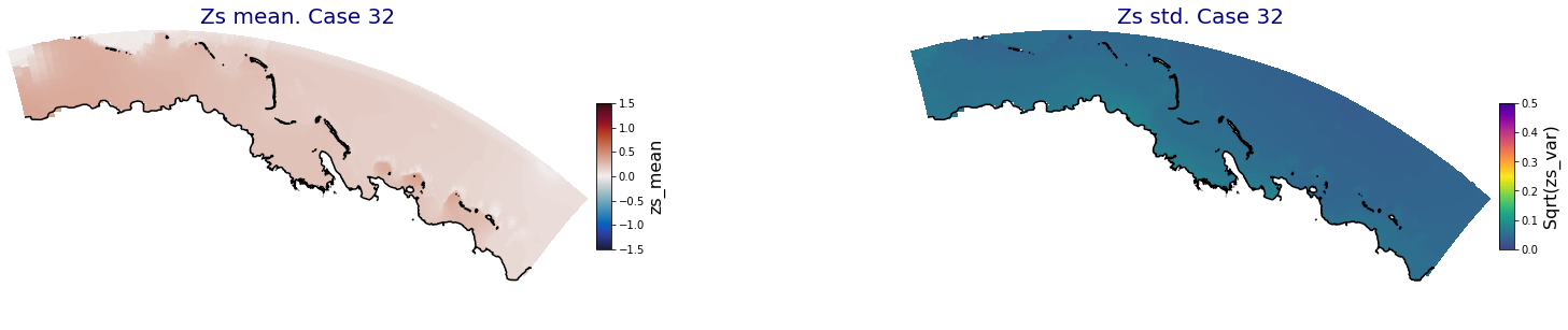
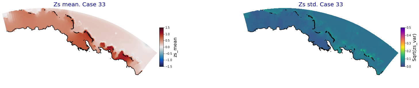
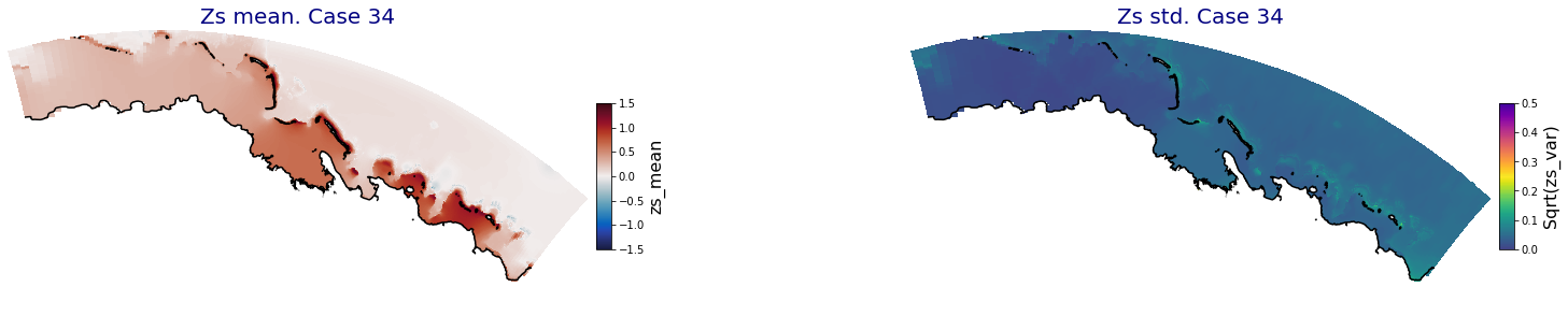
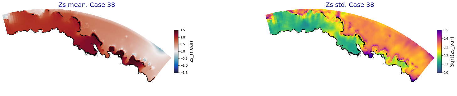
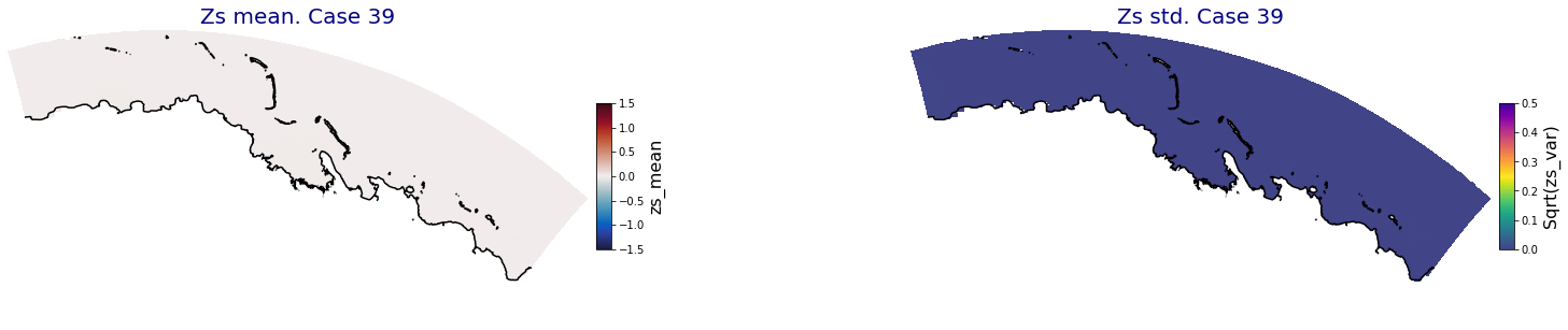
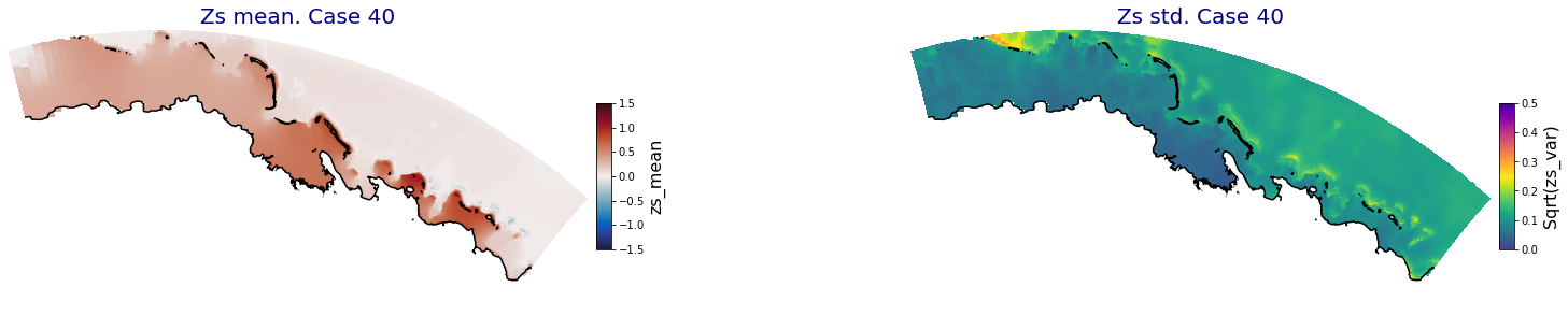
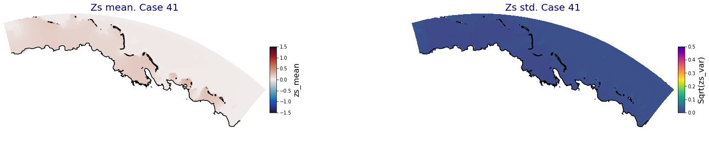
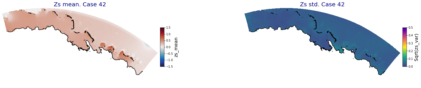
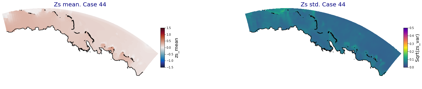
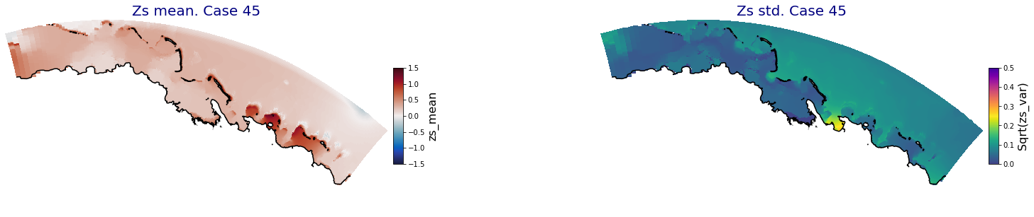
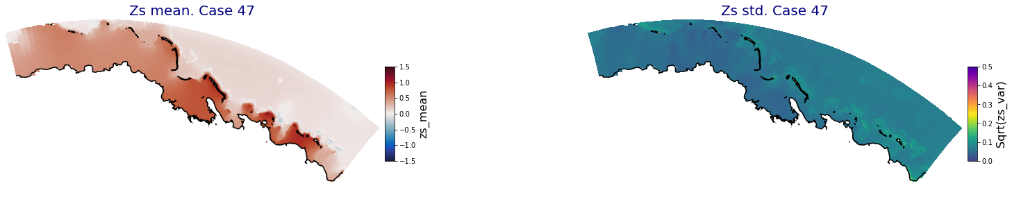
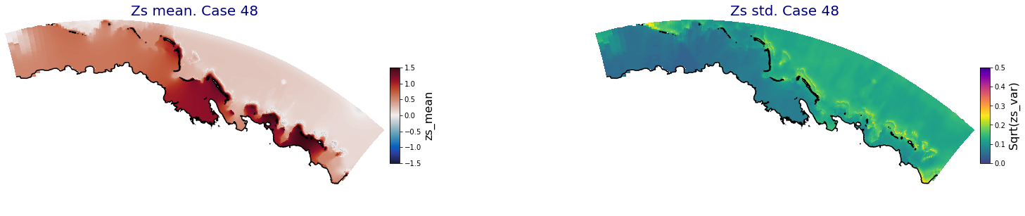
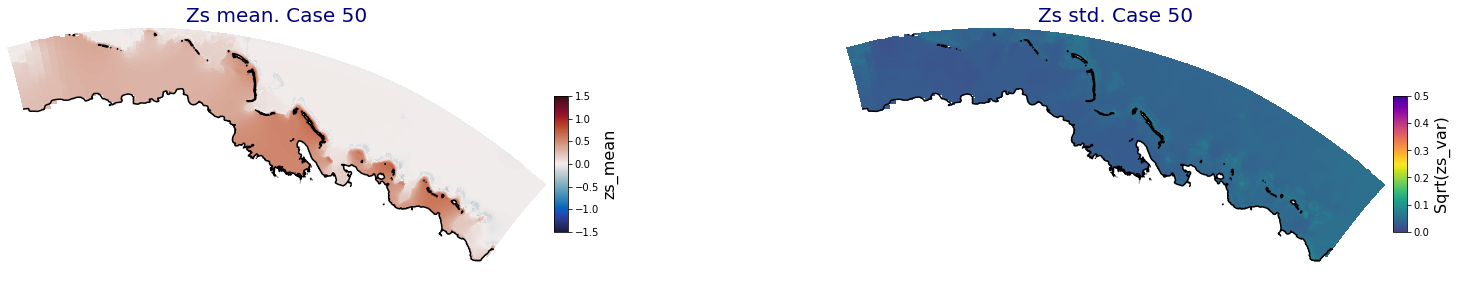
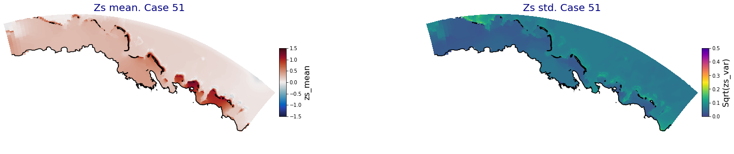
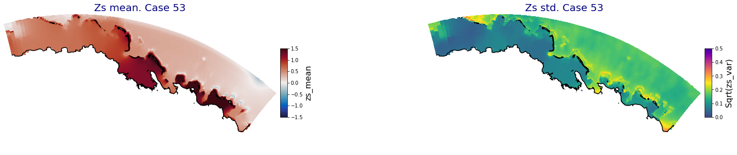
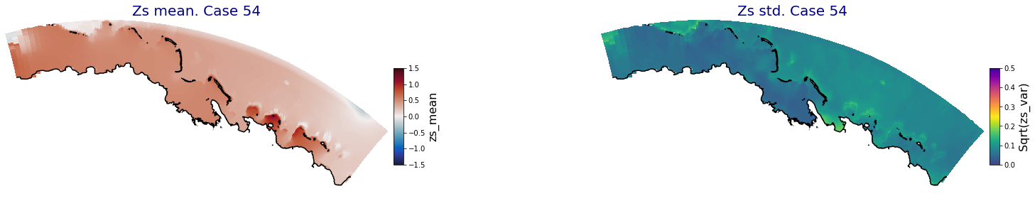
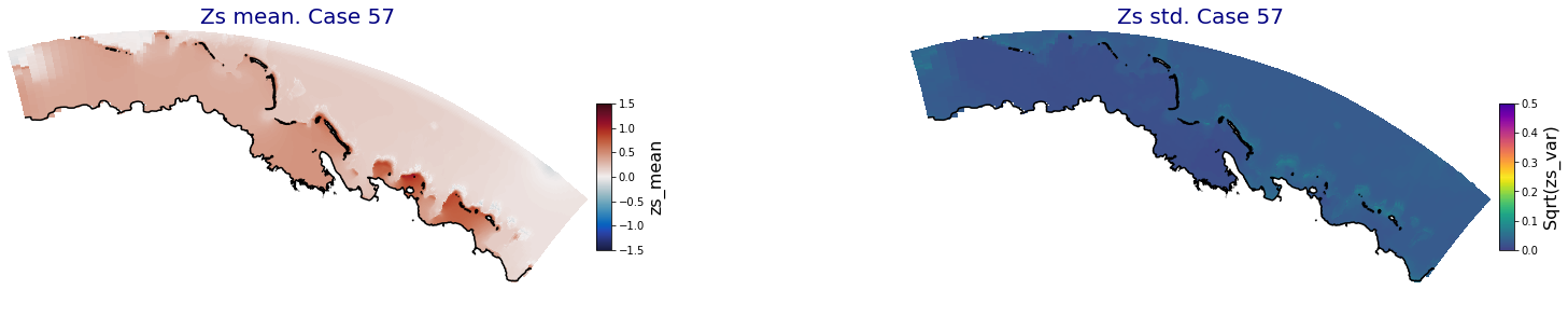
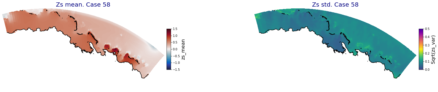
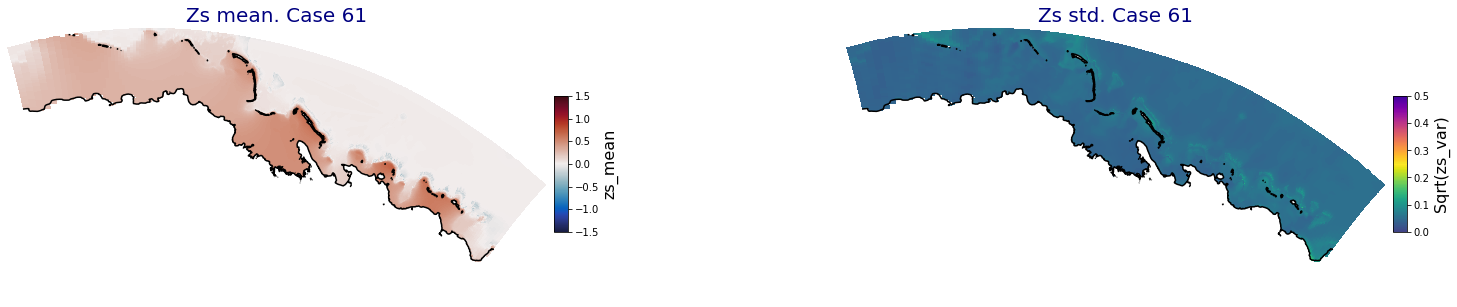
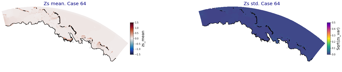
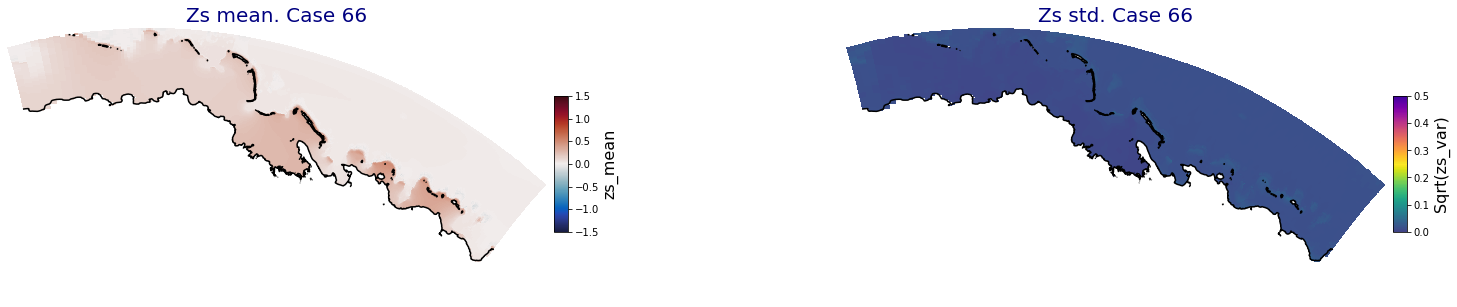
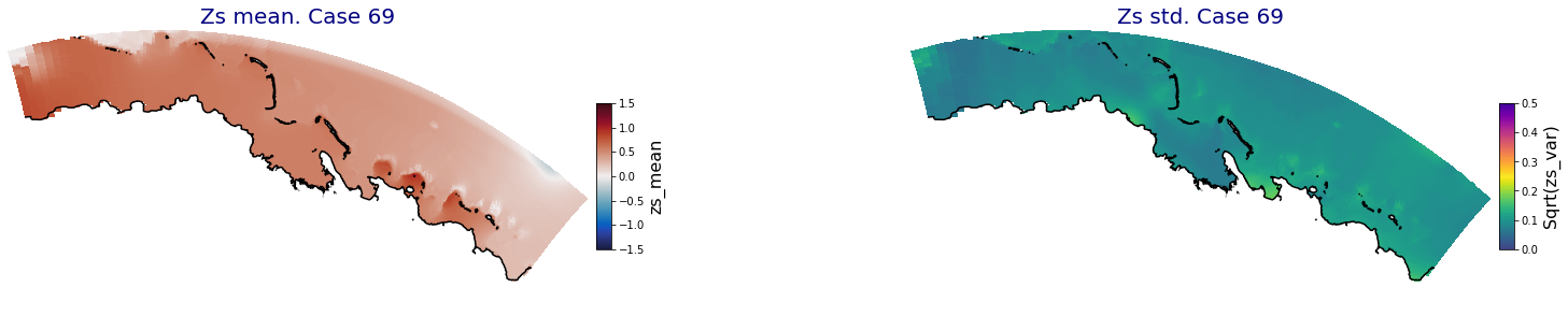
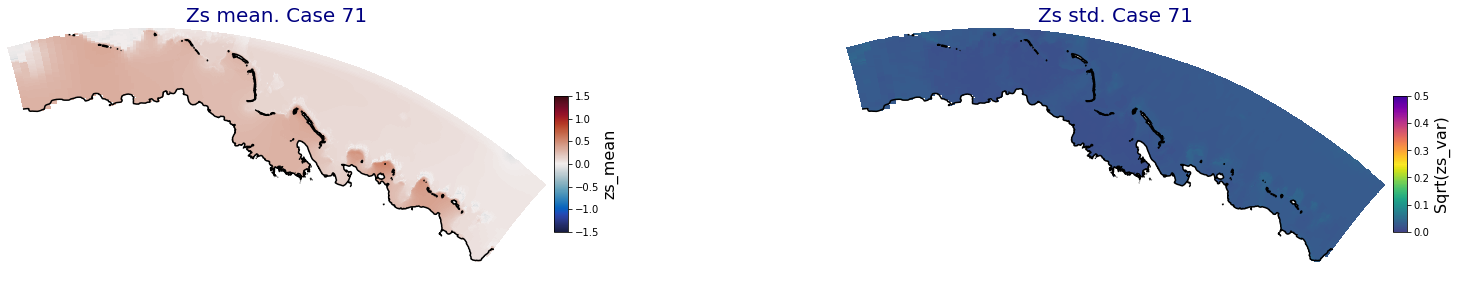
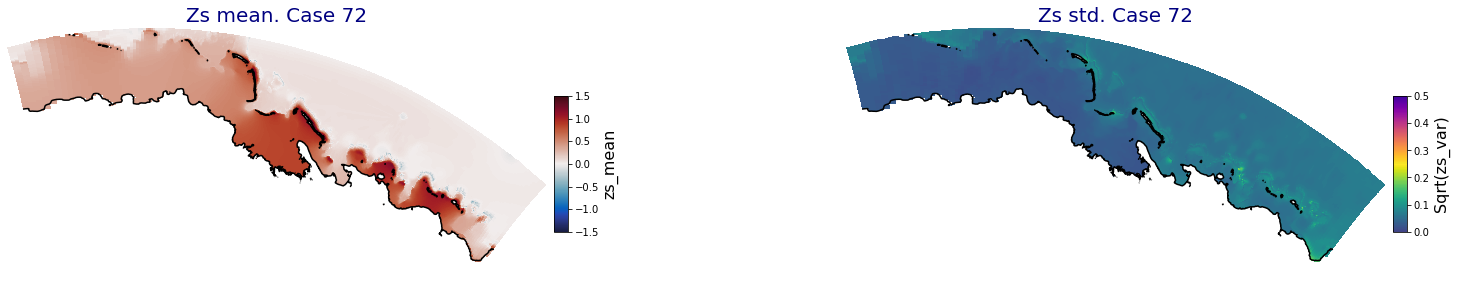
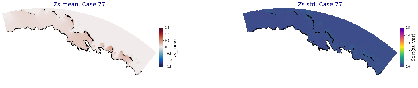
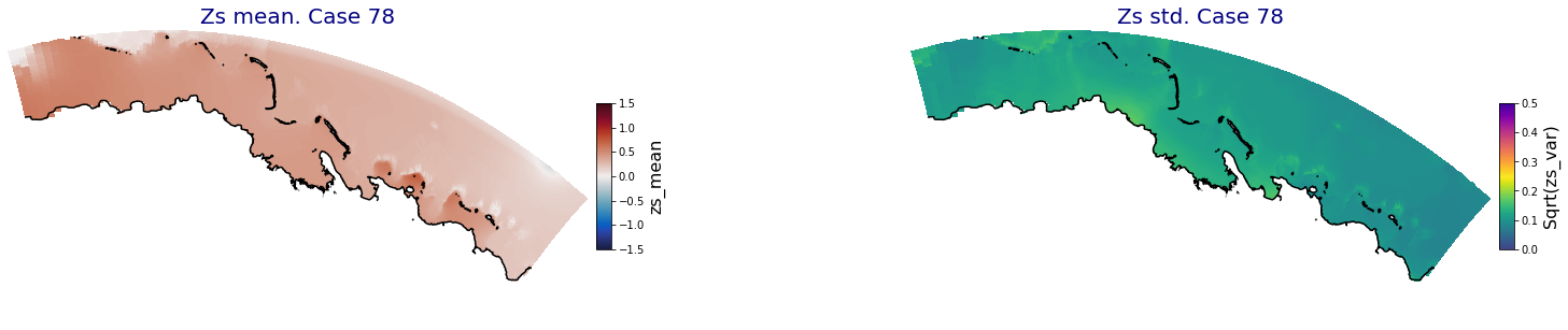
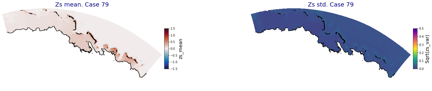
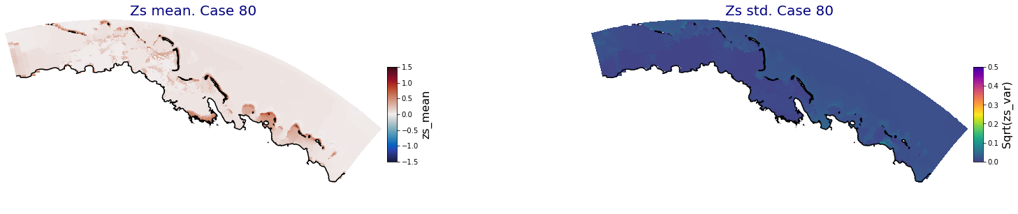
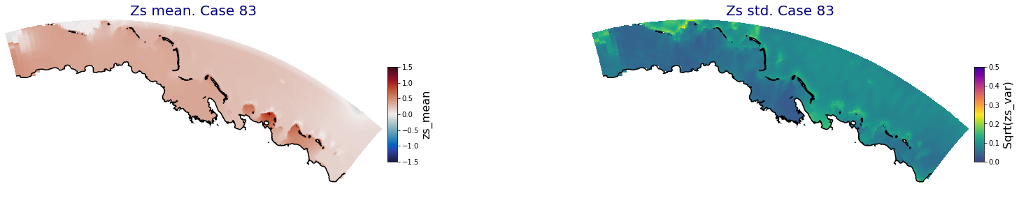
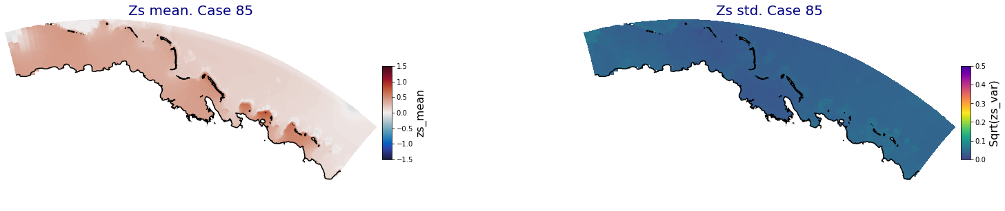
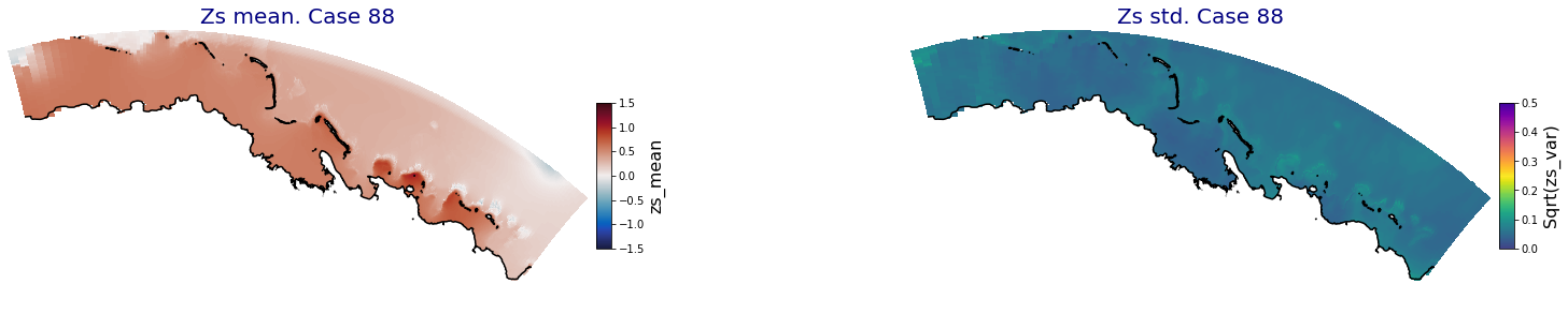
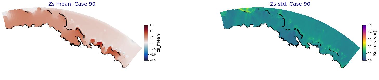
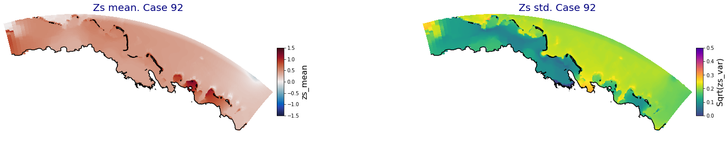
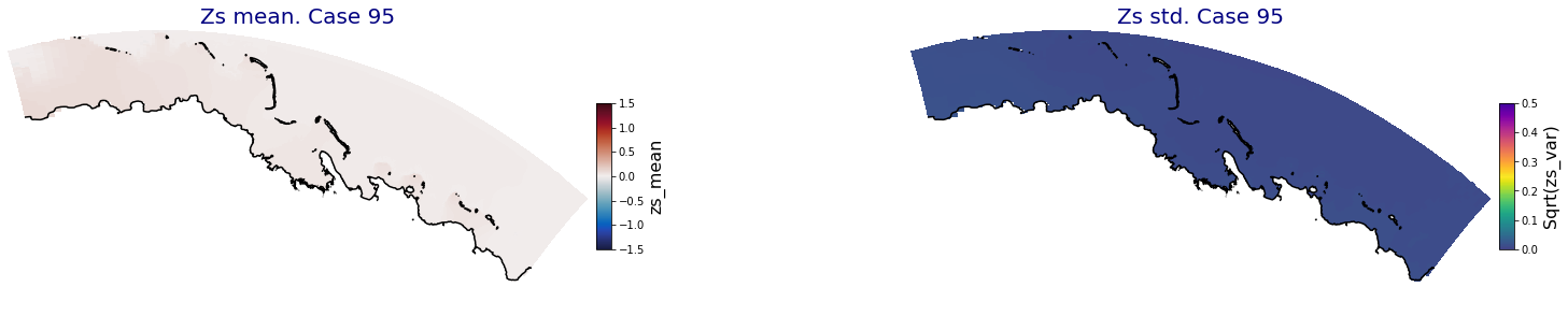
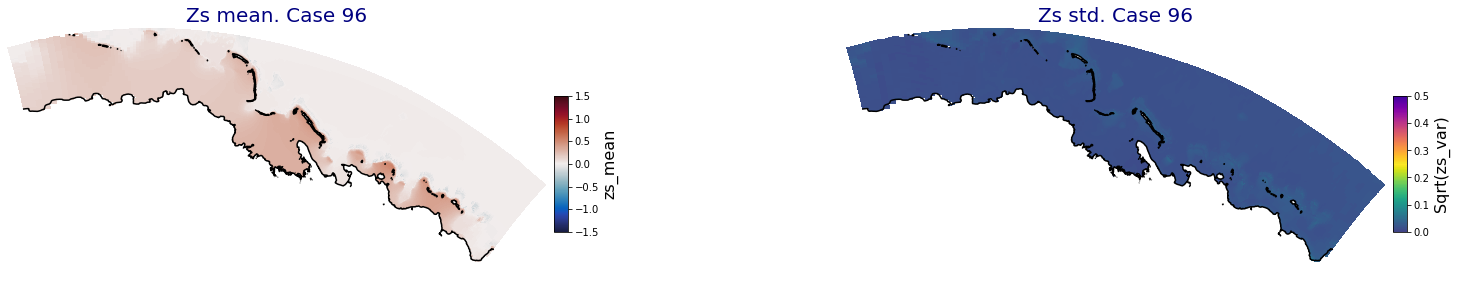
for i in range(ncases):
    
    fig = plt.figure(figsize=[30,5])
    gs = gridspec.GridSpec(1,2, hspace = 0.005, wspace = 0.005)
    ax = fig.add_subplot(gs[0])
    ax.set_title('Zs mean. Case '+str(i), fontsize=20, color='navy')
    
    Plot_Maps_XBeach(C_R_zs_mean.isel(case=i), vmin=-1.5, vmax=1.5, var_name = 'zs_mean',p_coast =1, ax=ax)

    
    ax = fig.add_subplot(gs[1])
    ax.set_title('Zs std. Case '+str(i), fontsize=20, color='navy')
    Plot_Maps_XBeach(C_R_zs_var.isel(case=i), vmin=0, vmax=0.5, var_name = 'zs_var',p_coast =1, ax=ax)

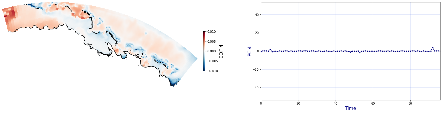
Principal Component Analysis (PCA)

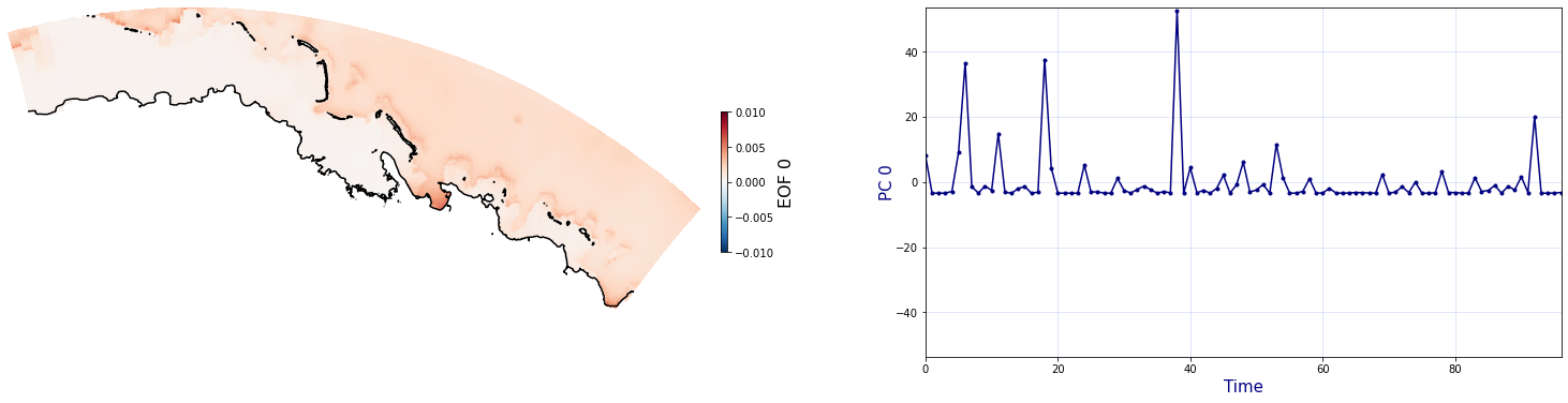
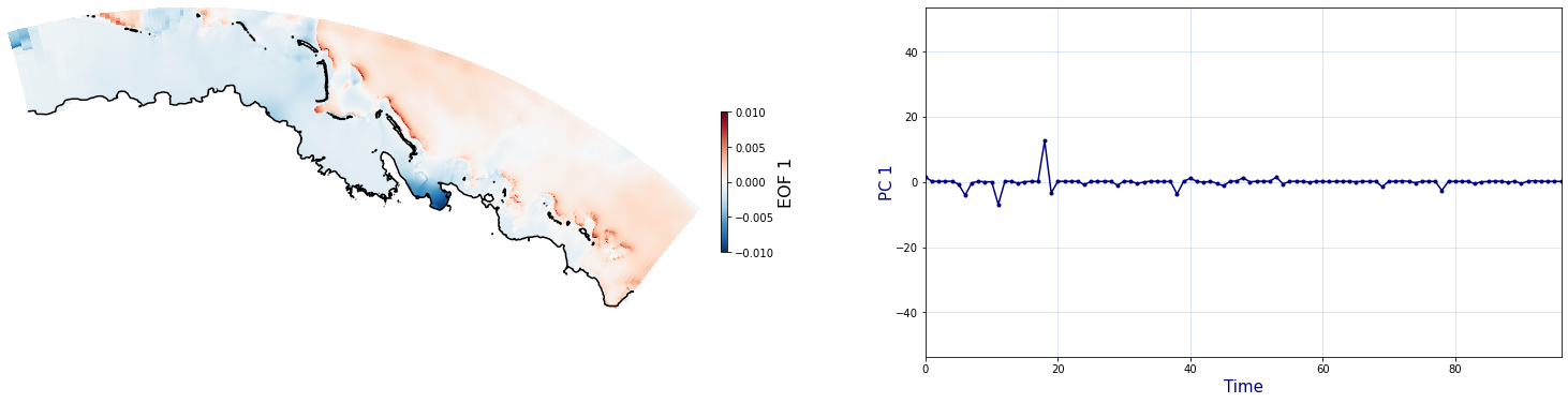
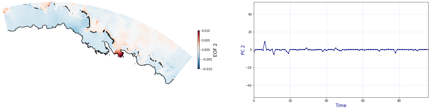
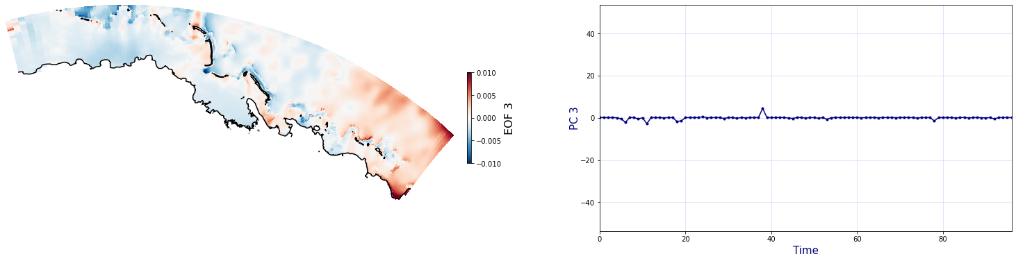
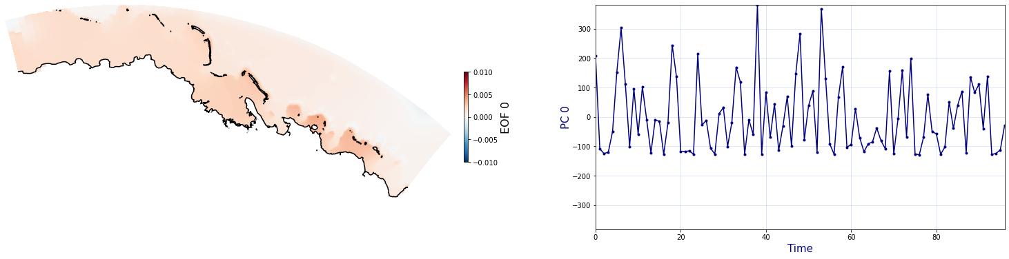
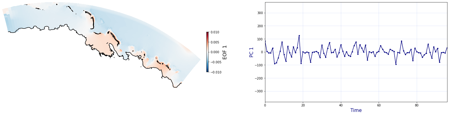
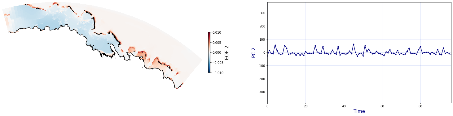
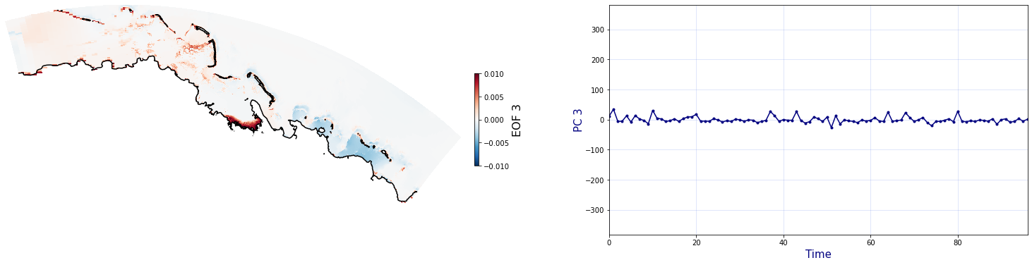
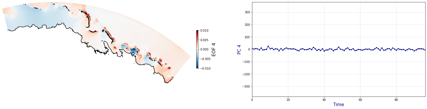
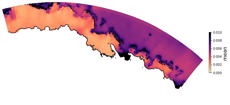
The Principal Component Analysis (PCA) is applied to the hourly fields of mean wave setup and its standard deviation to infer the infragravity wave component. This statistical technique is widely used in climatology to identify dominant variability patterns and reduce dimensionality (Camus et al. 2014). Hence, by PCA the main variability modes (patterns) of the target variables and the temporal coefficients of the identified patterns. PCA projects the original data on a new space, searching for the maximum variance of the sample data. The eigenvectors (empirical orthogonal functions, EOFs) of the data covariance matrix define the vectors of the new space. The transformed components of the original data over the new vectors are the principal components (PCs). Then, the target variables can be expressed as a linear combination of EOFs and PCs. As an example, following figure shows the first five empirical EOFs and PCs of the mean wave setup variable for one of the computational domains of Upolu, Apia region. Finally, the spatial and temporal reconstruction of these variables for any given sea state are obtained using this linear combination of EOFs and PCs combined with a non-linear interpolation technique based on radial basis functions (RBFs). This interpolation technique is very convenient for scattered and multivariate data (see details in Camus et al., 2011b).

HyBeat

The following intermediate results are for Apia domain in Upolu island

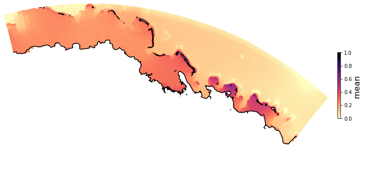
PCA of mean wave setup

Plot_EOFsMEAN(C_R_zs_mean, vmin=0, vmax=1,mask=1)

for n_pc in range(C_R_zs_mean.n_pcs.values):
    Plot_EOFs(C_R_zs_mean, n_pc=n_pc, vmin=-0.01, vmax=0.01,mask=1)

PCA of standard deviation of wave setup

Plot_EOFsMEAN(C_R_zs_var, vmin=0, vmax=0.01,mask=1)

for n_pc in range(C_R_zs_mean.n_pcs.values):
    Plot_EOFs(C_R_zs_var, n_pc=n_pc, vmin=-0.01, vmax=0.01,mask=1)