KMA Reconstruction
Contents
KMA Reconstruction#
# common
import warnings
warnings.filterwarnings('ignore')
import os
import os.path as op
import sys
import pickle as pkl

# pip
import xarray as xr
import numpy as np
import pandas as pd
import matplotlib.pyplot as plt

# DEV: bluemath
sys.path.insert(0, op.join(op.abspath(''), '..', '..', '..', '..'))

# bluemath modules
from bluemath.binwaves.reconstruction import generate_kp_coefficients, reconstruct_kmeans_clusters_hindcast

from bluemath.binwaves.plotting.swan_case import Plot_swan_case
from bluemath.binwaves.plotting.buoy import Plot_comparison_buoy, Plot_buoy_location
from bluemath.binwaves.plotting.spectra import Plot_example_spectra, Plot_spectra_propagation
Warning: cannot import cf-json, install "metocean" dependencies for full functionality
Database and site parameters#
# database
p_data = '/media/administrador/HD2/SamoaTonga/data'
p_site = op.join(p_data, 'Samoa')

# deliverable folder
p_deliv = op.join(p_site, 'd05_swell_inundation_forecast')

p_kma = op.join(p_deliv, 'kma')
p_swan = op.join(p_deliv, 'swan')

# SWAN simulation parameters
name = 'binwaves'
p_swan_subset = op.join(p_swan, name, 'subset.nc')
p_swan_output = op.join(p_swan, name, 'out_main_binwaves.nc')
p_swan_input_spec = op.join(p_swan, name, 'input_spec.nc')

# SuperPoint KMeans
num_clusters = 2000
p_superpoint_kma = op.join(p_kma, 'Spec_KMA_{0}_NS.nc'.format(num_clusters))

# buoy data
point_buoy = [187.8, -13.88]
p_buoy = op.join(p_site, 'buoy', 'samoaapolima_lon{0}_lat{1}_year1989_1990.pkl'.format(point_buoy[0], point_buoy[1]))


# output files
p_site_out = op.join(p_deliv, 'reconstruction')

p_kp_coeffs = op.join(p_site_out, 'kp_grid')          # SWAN propagation coefficients
p_efth_kma = op.join(p_site_out, 'efth_kma')          # KMA reconstruction
p_reco_hnd = op.join(p_site_out, 'hindcast')          # hindcast reconstruction folder
# aux functions

def load_point_kp(point, out_sim, p_kp_coeffs):
    '''
    Load kp propagation coefficients for a choosen point

    point   - point to load [lon, lat] (find nearest)
    out_sim - SWAN simulation output
    '''

    # find point
    ilon = np.argmin(np.abs(out_sim.lon.values - point[0]))
    ilat = np.argmin(np.abs(out_sim.lat.values - point[1]))

    # load coefficient
    fn = 'kp_lon_{0}_lat_{1}.nc'.format(out_sim.lon.values[ilon], out_sim.lat.values[ilat])
    p_cf = op.join(p_kp_coeffs, fn)

    return xr.open_dataset(p_cf)

def load_point_efth_kma(point, out_sim, p_efth):
    '''
    Load spectra efth_kma for a choosen point

    point - point to load [lon, lat] (find nearest)
    out_sim - SWAN simulation output
    '''

    # find point
    ilon = np.argmin(np.abs(out_sim.lon.values - point[0]))
    ilat = np.argmin(np.abs(out_sim.lat.values - point[1]))

    # load coefficient
    fn = 'efth_lon_{0}_lat_{1}.nc'.format(out_sim.lon.values[ilon], out_sim.lat.values[ilat])
    p_cf = op.join(p_efth, fn)

    return xr.open_dataset(p_cf)

def load_hindcast_recon(point, out_sim, p_reco):
    '''
    Load hindcast reconstruction for a choosen point

    point - point to load [lon, lat] (find nearest)
    out_sim - SWAN simulation output
    '''

    # find point
    ilon = np.argmin(np.abs(out_sim.lon.values - point[0]))
    ilat = np.argmin(np.abs(out_sim.lat.values - point[1]))

    # load coefficient
    fn = 'reconst_hind_lon_{0}_lat_{1}.nc'.format(out_sim.lon.values[ilon], out_sim.lat.values[ilat])
    p_cf = op.join(p_reco, fn)

    return xr.open_dataset(p_cf)
SWAN simulations and area#
SWAN Simulation parameters
# Load SWAN simulation parameters
subset = xr.open_dataset(p_swan_subset)
out_sim_swan = xr.open_dataset(p_swan_output)
input_spec = xr.open_dataset(p_swan_input_spec)
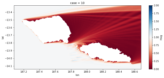
Here we need to define the area for the extraction and the resample factor
The plot is an example of the area that has been cut
# this will reduce memory usage
area_extraction = [-172.92+360, -171.3+360, -14.14, -13.3]
resample_factor = 2 #1 means no resample

# cut area
out_sim = out_sim_swan.sel(
    lon = slice(area_extraction[0], area_extraction[1]),
    lat = slice(area_extraction[2], area_extraction[3]),
)

# resample extraction points
out_sim = out_sim.isel(
    lon = np.arange(0, len(out_sim.lon), resample_factor),
    lat = np.arange(0, len(out_sim.lat), resample_factor),
)

# check that the area is OK
plt.figure(figsize = [12, 5])
out_sim.isel(case = 10).Hsig.plot(cmap='RdBu', vmin=0, vmax=2);
out_sim
<xarray.Dataset>
Dimensions:      (case: 696, lat: 138, lon: 267, partition: 10)
Coordinates:
  * lon          (lon) float64 187.1 187.1 187.1 187.1 ... 188.7 188.7 188.7
  * lat          (lat) float64 -14.14 -14.13 -14.13 ... -13.33 -13.32 -13.32
  * case         (case) int64 0 1 2 3 4 5 6 7 ... 689 690 691 692 693 694 695
Dimensions without coordinates: partition
Data variables:
    Tp           (case, lat, lon) float32 ...
    Dir          (case, lat, lon) float32 ...
    Tm02         (case, lat, lon) float32 ...
    Hsig         (case, lat, lon) float32 ...
    Dspr         (case, lat, lon) float32 ...
    Hs_part      (case, partition, lat, lon) float32 ...
    Tp_part      (case, partition, lat, lon) float32 ...
    Dir_part     (case, partition, lat, lon) float32 ...
    Dspr_part    (case, partition, lat, lon) float32 ...
count_parts (case, lat, lon) float64 ...- case: 696
- lat: 138
- lon: 267
- partition: 10
- lon(lon)float64187.1 187.1 187.1 ... 188.7 188.7
array([187.080835, 187.086835, 187.092835, ..., 188.664835, 188.670835, 188.676835]) - lat(lat)float64-14.14 -14.13 ... -13.32 -13.32
array([-14.137378, -14.131378, -14.125378, -14.119378, -14.113378, -14.107378, -14.101378, -14.095378, -14.089378, -14.083378, -14.077378, -14.071378, -14.065378, -14.059378, -14.053378, -14.047378, -14.041378, -14.035378, -14.029378, -14.023378, -14.017378, -14.011378, -14.005378, -13.999378, -13.993378, -13.987378, -13.981378, -13.975378, -13.969378, -13.963378, -13.957378, -13.951378, -13.945378, -13.939378, -13.933378, -13.927378, -13.921378, -13.915378, -13.909378, -13.903378, -13.897378, -13.891378, -13.885378, -13.879378, -13.873378, -13.867378, -13.861378, -13.855378, -13.849378, -13.843378, -13.837378, -13.831378, -13.825378, -13.819378, -13.813378, -13.807378, -13.801378, -13.795378, -13.789378, -13.783378, -13.777378, -13.771378, -13.765378, -13.759378, -13.753378, -13.747378, -13.741378, -13.735378, -13.729378, -13.723378, -13.717378, -13.711378, -13.705378, -13.699378, -13.693378, -13.687378, -13.681378, -13.675378, -13.669378, -13.663378, -13.657378, -13.651378, -13.645378, -13.639378, -13.633378, -13.627378, -13.621378, -13.615378, -13.609378, -13.603378, -13.597378, -13.591378, -13.585378, -13.579378, -13.573378, -13.567378, -13.561378, -13.555378, -13.549378, -13.543378, -13.537378, -13.531378, -13.525378, -13.519378, -13.513378, -13.507378, -13.501378, -13.495378, -13.489378, -13.483378, -13.477378, -13.471378, -13.465378, -13.459378, -13.453378, -13.447378, -13.441378, -13.435378, -13.429378, -13.423378, -13.417378, -13.411378, -13.405378, -13.399378, -13.393378, -13.387378, -13.381378, -13.375378, -13.369378, -13.363378, -13.357378, -13.351378, -13.345378, -13.339378, -13.333378, -13.327378, -13.321378, -13.315378]) - case(case)int640 1 2 3 4 5 ... 691 692 693 694 695
array([ 0, 1, 2, ..., 693, 694, 695])
- Tp(case, lat, lon)float32...
- units :
- s
- description :
- Waves Peak Period
[25644816 values with dtype=float32]
- Dir(case, lat, lon)float32...
- units :
- º
- description :
- Waves Direction
[25644816 values with dtype=float32]
- Tm02(case, lat, lon)float32...
- units :
- s
- description :
- Waves Mean Period
[25644816 values with dtype=float32]
- Hsig(case, lat, lon)float32...
[25644816 values with dtype=float32]
- Dspr(case, lat, lon)float32...
- units :
- º
- description :
- Waves Directional Spread
[25644816 values with dtype=float32]
- Hs_part(case, partition, lat, lon)float32...
[256448160 values with dtype=float32]
- Tp_part(case, partition, lat, lon)float32...
- units :
- s
- description :
- Partition of Waves Peak Period
[256448160 values with dtype=float32]
- Dir_part(case, partition, lat, lon)float32...
- units :
- º
- description :
- Partition of Waves Direction
[256448160 values with dtype=float32]
- Dspr_part(case, partition, lat, lon)float32...
- units :
- º
- description :
- Partition of directional spread
[256448160 values with dtype=float32]
- count_parts(case, lat, lon)float64...
[25644816 values with dtype=float64]
KMA clusters#
We reconstruct the spec in the grid points, for the 2000 spectral centroids of the cluster
sp_kma = xr.open_dataset(p_superpoint_kma)
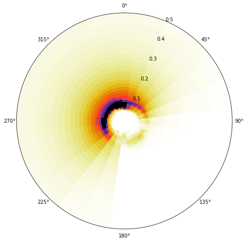
One cluster example OFFSHORE
# example cluster
cluster = 4

# Plot spectra
Plot_example_spectra(sp_kma, cluster=cluster);
Simulations preprocess#
This is where we postprocess all the simulations, to obtain the propagation coefficients (kp) for all the 696 cases and for each point of the grid
This process takes a long time but it only needs to be run once
# generate propagation coefficients for all points and cases
generate_kp_coefficients(p_kp_coeffs, out_sim, sp_kma, override=False)
Preprocessing kp coefficients...: 100%|██████████████████████████████| 36846/368
Explanation
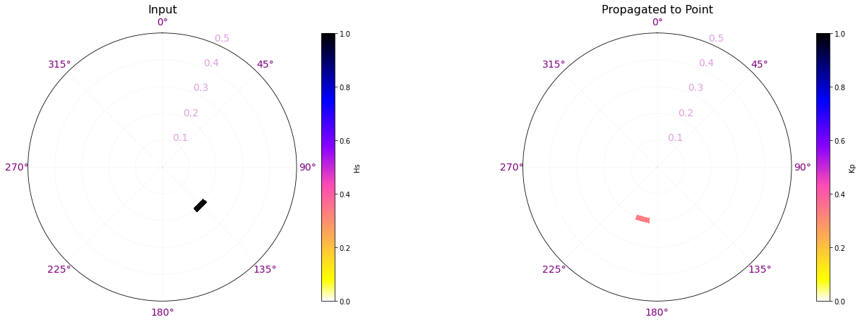
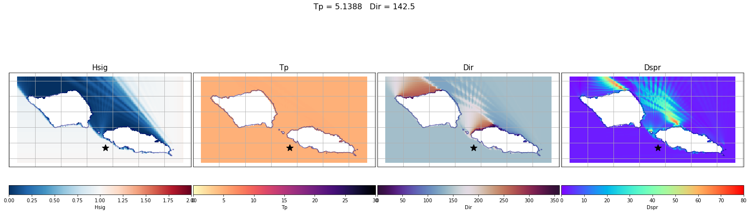
Here are a couple examples of the process made here for one of the propagation cases.
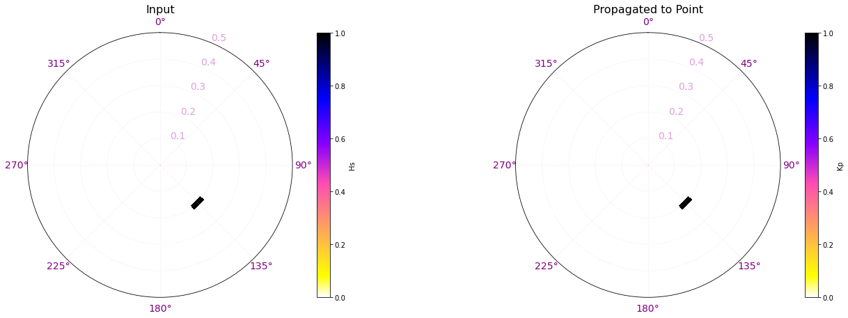
In the plots below, the propagation for a case out of the 696 has been plotted with the propagations for two different points of the grid (The ones marked with a star)
The first example is for the buoy location, which receives all the energy from the 142.5º direction. The Kp coefficient is 1 with the same direction as the input offshore spectra, meaning that any energy is lost.
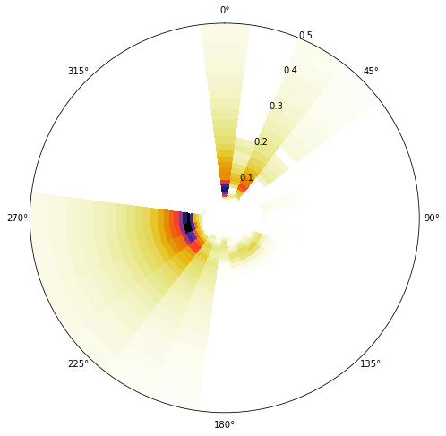
The second example is for a location in the northern part of Tognatapu, where waves are shadowed by the many small islands in the area. For this reason the same input spectra is here transformed into 4 different systems with different directions, kist a kp coefficient of around 0.1/0.2
# Select one propagation case
case = 250
point_example = [187.93, -13.76]

# Load spectra kp
output_spec = load_point_kp(point_example, out_sim, p_kp_coeffs)

# Plot SWAN case
Plot_swan_case(out_sim, subset, case, point_example[0], point_example[1]);

# Plot SWAN Hs propagation spectra
Plot_spectra_propagation(input_spec, output_spec, sp_kma, case, ylim=0.5, cmap='gnuplot2_r');

# Select one propagation case
case = 250
point_example = [187.93, -14.00]

# Load spectra kp
output_spec = load_point_kp(point_example, out_sim, p_kp_coeffs)

# Plot SWAN case
Plot_swan_case(out_sim, subset, case, point_example[0], point_example[1]);

# Plot SWAN Hs propagation spectra
Plot_spectra_propagation(input_spec, output_spec, sp_kma, case, ylim=0.5, cmap='gnuplot2_r');
Reconstruction based on KMA#
Validation#
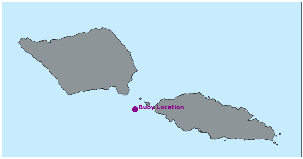
Below is the Buoy Location available for validation at our study site
# Plot buoy location
Plot_buoy_location(point_buoy, area_extraction);
Buoy Location 1#
# reconstruct model data for that specific point
reconstruct_kmeans_clusters_hindcast(
    p_site_out, out_sim, sp_kma,
    point = point_buoy,
    reconst_hindcast = True,
    override = False,
)
Preprocessing efth and stats...: 100%|██████████████████████████████| 1/1 [00:23
Same cluster as in the example above, propagated to buoy at Location 1
# Load propagated spectra
efth_point = load_point_efth_kma(point_buoy, out_sim, p_efth_kma)

# Plot spectra
Plot_example_spectra(efth_point, cluster=cluster);
# load buoy data and parse it to xarray.Dataset
with open(p_buoy, 'rb') as fr:
    buoy = pkl.load(fr)

buoy_data = buoy.to_xarray().isel(index = np.where((buoy.hs > 0) & (buoy.tm10 > 0))[0])
# Load hindcast reconstruction at nearest point to buoy
recon_data = load_hindcast_recon(point_buoy, out_sim, p_reco_hnd)
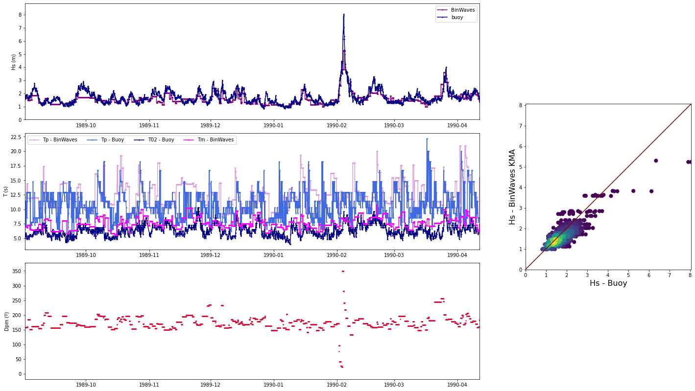
# compare hindcast reconstruction with buoy data
Plot_comparison_buoy(recon_data, buoy_data, ss=3);