Rainfall Model
Contents
Rainfall Model#
import warnings
warnings.filterwarnings('ignore')
import os
import os.path as op
import sys

import matplotlib.pyplot as plt
import xarray as xr
import pandas as pd
import numpy as np
import geopandas as gpd
import utm
sys.path.insert(0, os.path.join(os.path.abspath(''), '..','..', '..' ))

from bluemath.rainfall_forecast.rainfall_forecast import *
from bluemath.rainfall_forecast.graffiti_rain import *
Warning: cannot import cf-json, install "metocean" dependencies for full functionality
# database
p_data = r'/media/administrador/HD2/SamoaTonga/data'
site, site_, nm = 'Upolu', 'upolu', 'up'
p_site = op.join(p_data, site)

p_deliv = op.join(p_site, 'd09_rainfall_forecast')
p_figs = op.join(p_deliv, 'figs')

#Basins path
p_basins = op.join(p_deliv, 'basins', nm + '_db' +  '_fixed.shp')

#Som fitting
p_som_fit = os.path.join(p_deliv, 'som_fit_30x30_4d.nc')

#Parameters from classification
p_params_fit = os.path.join(p_deliv, 'params_fit_30x30_4d_clust.nc')

#Historical track
n = 166
p_hist_track = os.path.join(p_deliv,'sp_{0}.nc'.format(n))
times_sel = [150, 385] #Times to cut that specific track to our area

#output files
p_rain_out = os.path.join(p_deliv,'rain_sp_{0}.nc'.format(n))

# make data folders
for f in [p_deliv, p_figs]:
    if not op.isdir(f):
        os.makedirs(f)
#Parameters

area_interest = [[187.848, 188.63],[-14.078, -13.756]] #upolu
discretization = 0.05 #local grid discretization
bas_raw = gpd.read_file(p_basins)
Regional Scale#
A model to estimate rainfall caused by the action of tropical cyclones (TCs) according to atmospheric, geographical, and oceanic variables has been developed. For this purpose, three databases have been used: precipitation measured by satellite GPM mission with half-hourly temporal resolution and 0.1° of spatial resolution, TCs historical tracks from IBTrACS and sea surface temperature (SST) from the NOAA OI SST V2 High Resolution Dataset with daily data at 0.25° spatial resolution.
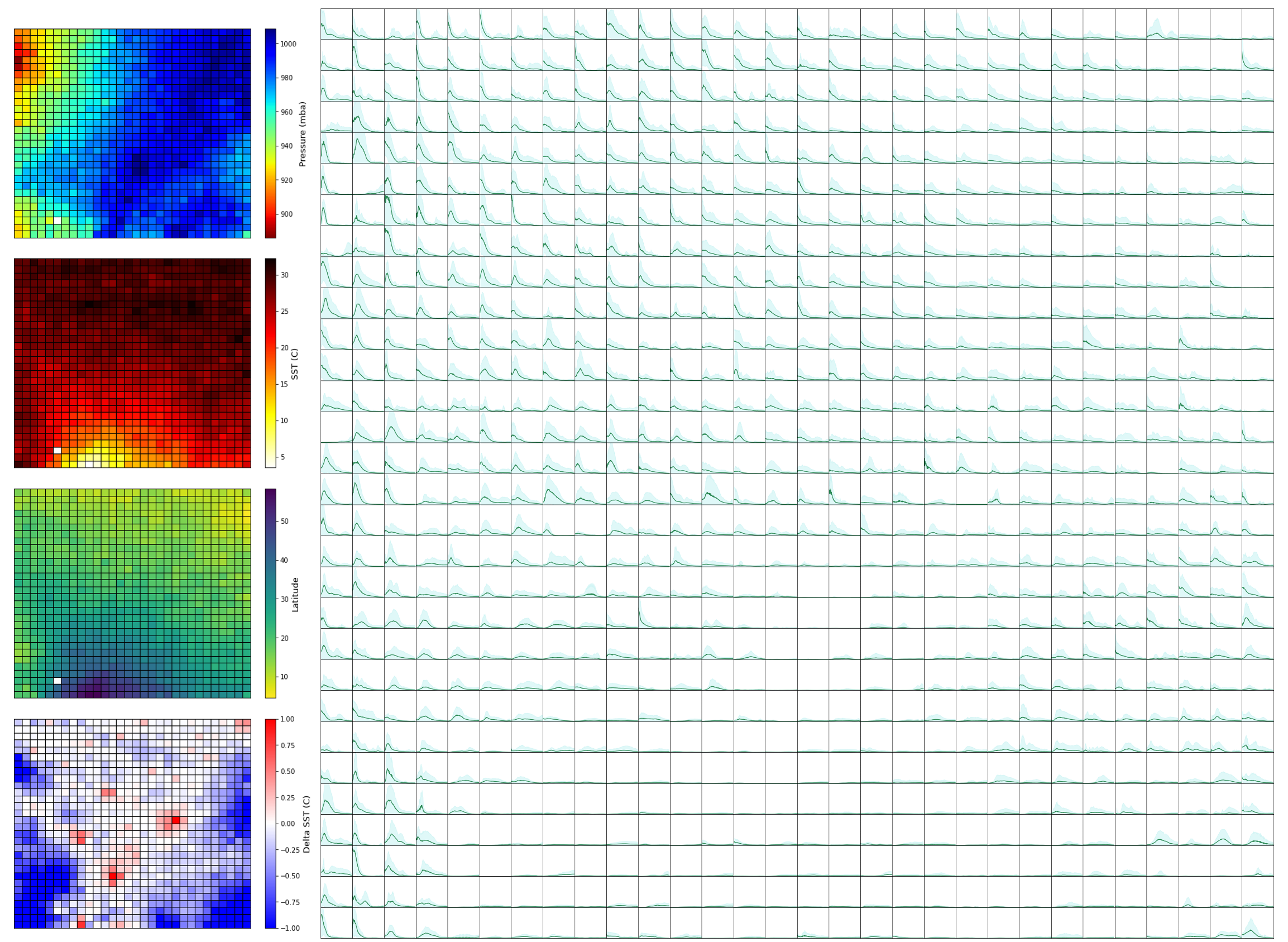
The model assumes a circular shape of the TC influence area and defines the precipitation clustered in 900 groups following a Self-Organizing Maps (SOM) algorithm as a function of:
TC track minimum pressure
TC track sea surface temperature
TC track latitude
\(\Delta\)SST : difference in sea surface temperature between the current day and the previous day averaged in an circular area of radius equal to 200 km from the TC track
For each of the 900 clusters, the mean precipitacion over the radius dimension is calculated, and the curves are shown below.
from IPython.display import Image
Image('./resources/Rainfall_SOM.png', width=1000)
Load needed files#
To run the model, we need to load the data corresponding to the SOM clustering (som_fit dataset) and the parameters associated to each of the 900 clusters (params_fit dataset).
som_fit = xr.open_dataset(p_som_fit)
params_fit = xr.open_dataset(p_params_fit)
Rainfall footprint#
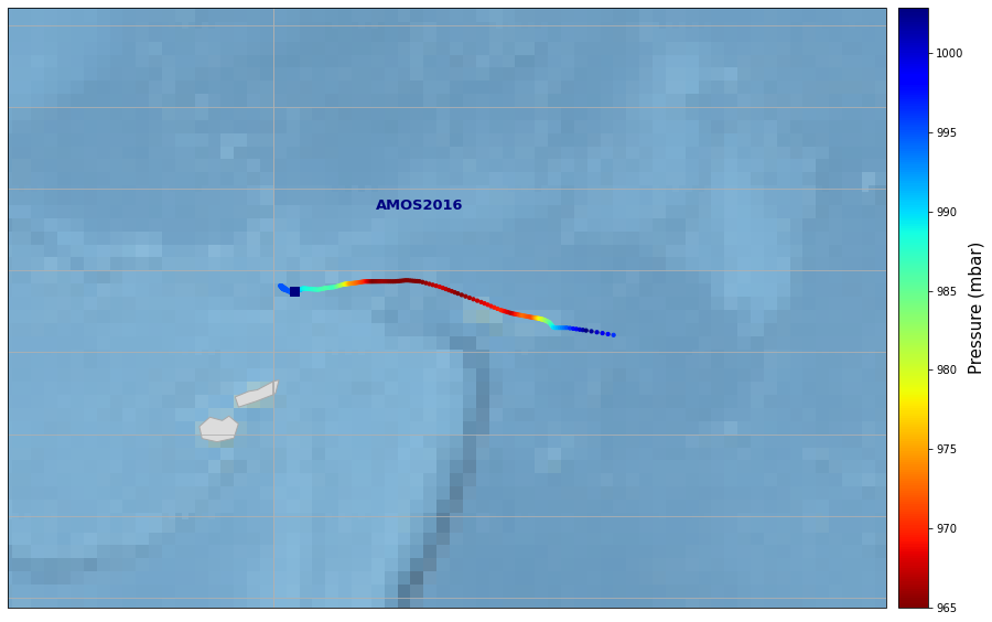
For a historical TC track:
tco = xr.open_dataset(p_hist_track)
tc = process_tc_file(tco)
TC: AMOS, starting day 2016-04-17
#We can select the dates we are interested in
tc = tc.isel(date_time=slice(times_sel[0], times_sel[1]))
Plot TC track
The track is coloured according to the minimum pressure value
fig_tc = Plot_track(tc, figsize=[20,10], cmap='jet_r', m_size=10)
Obtain rainfall fields
interp=1 #interp: 1:activate / 0:deactivate
interp_factor=1 #multiply by interp_factor the number of points along the track, in this case we already have the data each half hour in the TCs database
min_points=5 #minimum points to consider TC track and process it
tc_r = Generate_Rain_TC_4D(tc, som_fit, params_fit, interp, interp_factor, min_points)
time step 209
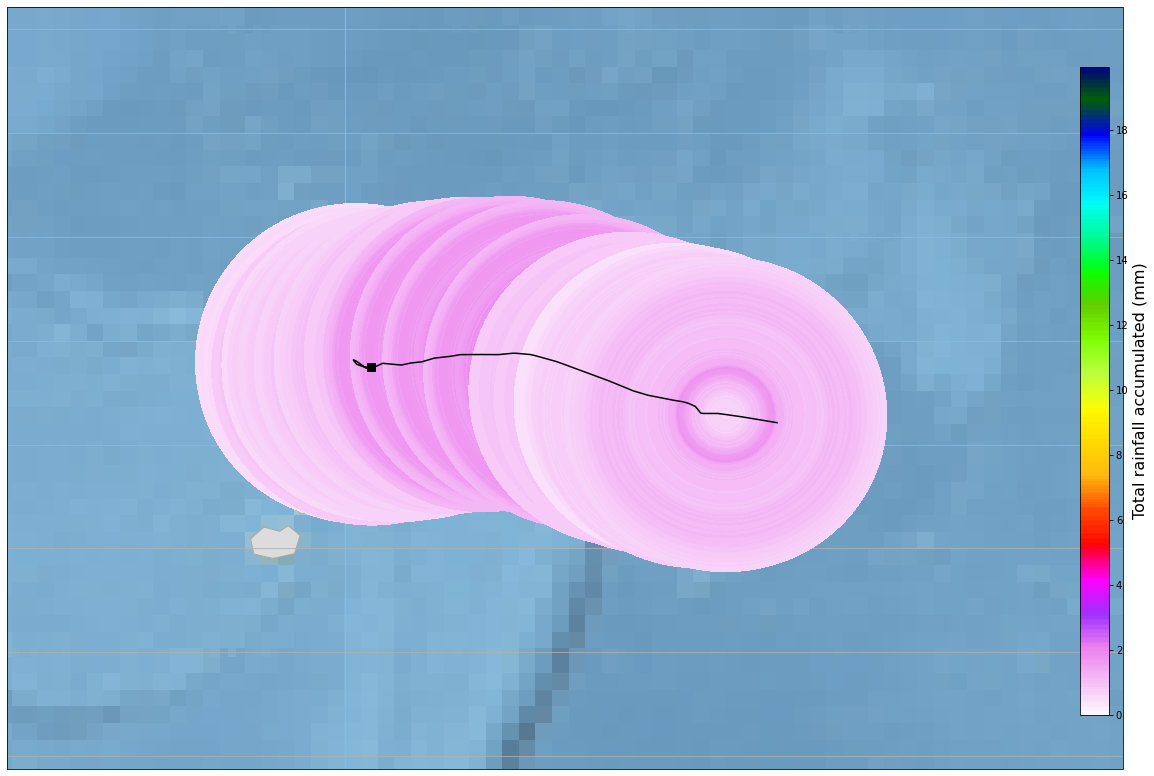
Once the model is constructed, from any TC track with its corresponding values of SST, latitude, minimum pressure and \(\Delta\)SST, a precipitation field from the closest cluster can be assigned to each position of the TC track.
Plot rain field
rmax = 20
figsize = [25,12]
fig_rf = plot_rain_fields(tc,tc_r,figsize,rmax)
Total storm rainfall#
Here we grid the results into a regular grid with the resolution given below (discretization), to obtain the resultant rainfall grid in mm/hr associated to each temporal moment.
Then we aggregate the results to obtain the resultant rainfall footprint for all the storm.
Obtain the grid for each temporal moment
discretization = 0.5
l_ds = tc_grid(tc_r,discretization)
time step 209
#Dataset containing for each temporal moment the resultant rainfall grid
dst = xr.concat(l_ds,dim='time')

#Dataset with the resultant rainfall footprint for all the TC duration
dss = dst.sum(dim='time')*0.5

dss.to_netcdf(p_rain_out)
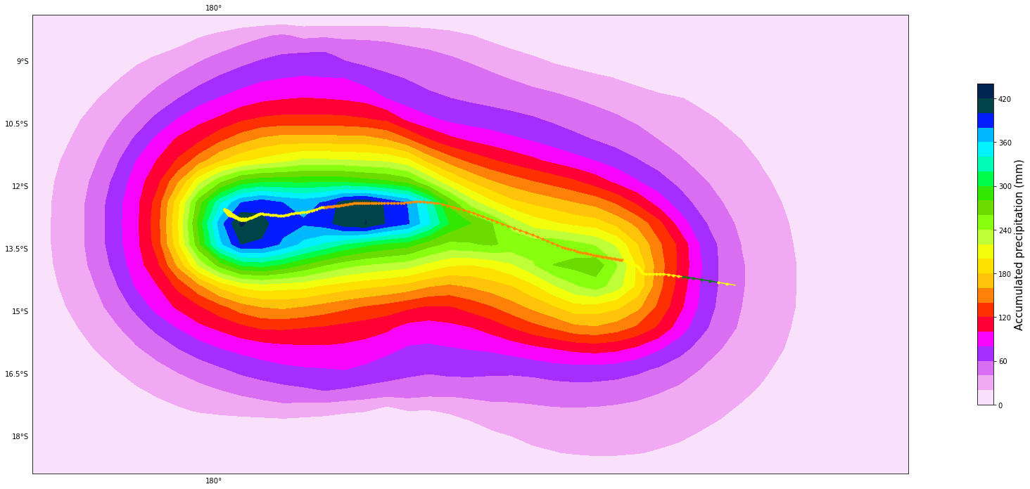
By aggregating the rainfall at each point of the region, the rainfall SWATH for the duration of the storm can be obtained
fig_total_storm_tc = tc_total_rain(tc, dss, figsize=[25,12])
Local Scale#
Define area of interest and gris parameters
area_interest_l = [[area_interest[0][0]-discretization*3, area_interest[0][1]+discretization*3],[area_interest[1][0]-discretization*3, area_interest[1][1]+discretization*3]] #upolu

l_ds_area = tc_grid(tc_r,discretization, area=area_interest_l)
dst_area = xr.concat(l_ds_area,dim='time')
dss_area = dst_area.sum(dim='time')*0.5
time step 209
dst_area = dst_area.interp(lon=np.arange(dss_area.lon[0], dss_area.lon[-1], 0.01), lat=np.arange(dss_area.lat[0], dss_area.lat[-1], 0.01), method='linear')
dst_area = dst_area.sel(lon=slice(area_interest[0][0], area_interest[0][1]), lat=slice(area_interest[1][0], area_interest[1][1]))
dss_area = dss_area.interp(lon=np.arange(dss_area.lon[0], dss_area.lon[-1], 0.01), lat=np.arange(dss_area.lat[0], dss_area.lat[-1], 0.01), method='linear')
dss_area = dss_area.sel(lon=slice(area_interest[0][0], area_interest[0][1]), lat=slice(area_interest[1][0], area_interest[1][1]))
dst_area
<xarray.Dataset>
Dimensions:      (lat: 32, lon: 78, time: 210)
Coordinates:
  * lon          (lon) float64 187.9 187.9 187.9 187.9 ... 188.6 188.6 188.6
  * lat          (lat) float64 -14.07 -14.06 -14.05 ... -13.78 -13.77 -13.76
Dimensions without coordinates: time
Data variables:
    rain         (time, lat, lon) float64 nan nan nan nan ... 1.301 1.306 1.31
cell_counts (time, lat, lon) float64 nan nan nan nan ... 84.97 85.23 85.48- lat: 32
- lon: 78
- time: 210
- lon(lon)float64187.9 187.9 187.9 ... 188.6 188.6
array([187.858, 187.868, 187.878, 187.888, 187.898, 187.908, 187.918, 187.928, 187.938, 187.948, 187.958, 187.968, 187.978, 187.988, 187.998, 188.008, 188.018, 188.028, 188.038, 188.048, 188.058, 188.068, 188.078, 188.088, 188.098, 188.108, 188.118, 188.128, 188.138, 188.148, 188.158, 188.168, 188.178, 188.188, 188.198, 188.208, 188.218, 188.228, 188.238, 188.248, 188.258, 188.268, 188.278, 188.288, 188.298, 188.308, 188.318, 188.328, 188.338, 188.348, 188.358, 188.368, 188.378, 188.388, 188.398, 188.408, 188.418, 188.428, 188.438, 188.448, 188.458, 188.468, 188.478, 188.488, 188.498, 188.508, 188.518, 188.528, 188.538, 188.548, 188.558, 188.568, 188.578, 188.588, 188.598, 188.608, 188.618, 188.628]) - lat(lat)float64-14.07 -14.06 ... -13.77 -13.76
array([-14.068, -14.058, -14.048, -14.038, -14.028, -14.018, -14.008, -13.998,
       -13.988, -13.978, -13.968, -13.958, -13.948, -13.938, -13.928, -13.918,
       -13.908, -13.898, -13.888, -13.878, -13.868, -13.858, -13.848, -13.838,
       -13.828, -13.818, -13.808, -13.798, -13.788, -13.778, -13.768, -13.758])
- rain(time, lat, lon)float64nan nan nan ... 1.301 1.306 1.31
array([[[ nan, nan, nan, ..., nan, nan, nan], [ nan, nan, nan, ..., nan, nan, nan], [ nan, nan, nan, ..., nan, nan, nan], ..., [ nan, nan, nan, ..., nan, nan, nan], [ nan, nan, nan, ..., nan, nan, nan], [ nan, nan, nan, ..., nan, nan, nan]], [[ nan, nan, nan, ..., nan, nan, nan], [ nan, nan, nan, ..., nan, nan, nan], [ nan, nan, nan, ..., nan, nan, nan], ... [0.93568498, 0.93957245, 0.94345993, ..., 1.14497477, 1.14569798, 1.1464212 ], [0.93568498, 0.93957245, 0.94345993, ..., 1.14497477, 1.14569798, 1.1464212 ], [0.93568498, 0.93957245, 0.94345993, ..., 1.14497477, 1.14569798, 1.1464212 ]], [[1.04987057, 1.05339143, 1.05691229, ..., 1.35071532, 1.35565081, 1.3605863 ], [1.04898148, 1.05249838, 1.05601528, ..., 1.34912484, 1.35404081, 1.35895679], [1.0480924 , 1.05160533, 1.05511827, ..., 1.34753435, 1.35243081, 1.35732727], ..., [1.024087 , 1.02749303, 1.03089907, ..., 1.30459129, 1.30896085, 1.31333041], [1.02319791, 1.02659998, 1.03000206, ..., 1.30300081, 1.30735085, 1.3117009 ], [1.02230882, 1.02570694, 1.02910505, ..., 1.30141033, 1.30574085, 1.31007138]]]) - cell_counts(time, lat, lon)float64nan nan nan ... 84.97 85.23 85.48
array([[[    nan,     nan,     nan, ...,     nan,     nan,     nan],
        [    nan,     nan,     nan, ...,     nan,     nan,     nan],
        [    nan,     nan,     nan, ...,     nan,     nan,     nan],
        ...,
        [    nan,     nan,     nan, ...,     nan,     nan,     nan],
        [    nan,     nan,     nan, ...,     nan,     nan,     nan],
        [    nan,     nan,     nan, ...,     nan,     nan,     nan]],

       [[    nan,     nan,     nan, ...,     nan,     nan,     nan],
        [    nan,     nan,     nan, ...,     nan,     nan,     nan],
        [    nan,     nan,     nan, ...,     nan,     nan,     nan],
        ...,
...
        ...,
        [78.036 , 78.272 , 78.508 , ..., 95.84  , 96.08  , 96.32  ],
        [78.0932, 78.3264, 78.5596, ..., 95.76  , 96.    , 96.24  ],
        [78.1504, 78.3808, 78.6112, ..., 95.68  , 95.92  , 96.16  ]],

       [[73.3172, 73.5944, 73.8716, ..., 92.6408, 92.8616, 93.0824],
        [73.3544, 73.6288, 73.9032, ..., 92.5616, 92.7832, 93.0048],
        [73.3916, 73.6632, 73.9348, ..., 92.4824, 92.7048, 92.9272],
        ...,
        [74.396 , 74.592 , 74.788 , ..., 90.344 , 90.588 , 90.832 ],
        [74.4332, 74.6264, 74.8196, ..., 90.2648, 90.5096, 90.7544],
        [74.4704, 74.6608, 74.8512, ..., 90.1856, 90.4312, 90.6768]],

       [[67.9648, 68.1896, 68.4144, ..., 86.2392, 86.5184, 86.7976],
        [67.7096, 67.9392, 68.1688, ..., 86.1984, 86.4768, 86.7552],
        [67.4544, 67.6888, 67.9232, ..., 86.1576, 86.4352, 86.7128],
        ...,
        [60.564 , 60.928 , 61.292 , ..., 85.056 , 85.312 , 85.568 ],
        [60.3088, 60.6776, 61.0464, ..., 85.0152, 85.2704, 85.5256],
        [60.0536, 60.4272, 60.8008, ..., 84.9744, 85.2288, 85.4832]]])
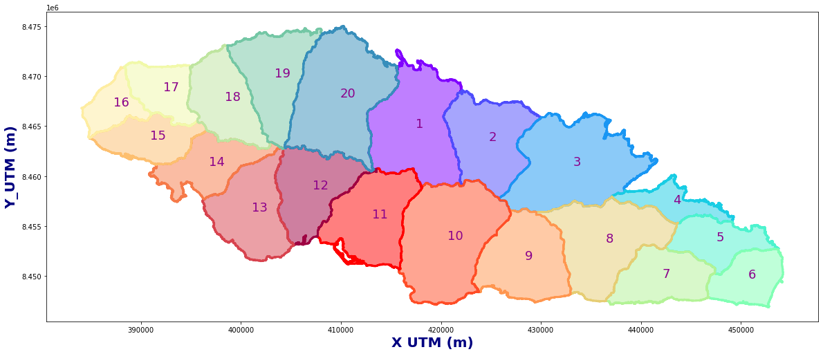
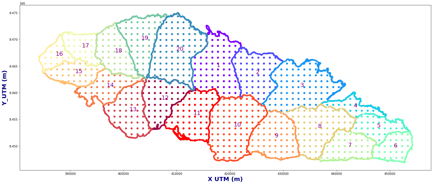
Basins discretization#
The discretization of the island in its watersheds have been carried out by means of QGIS, an open-source cross-platform desktop geographic information system (GIS) application that supports viewing, editing, and analysis of geospatial data. From the 5m resolution digital elevation model, a number of basins have been obtained, as in the following figure:
basins = Obtain_Basins(bas_raw, site)
Plot_Basins(basins)
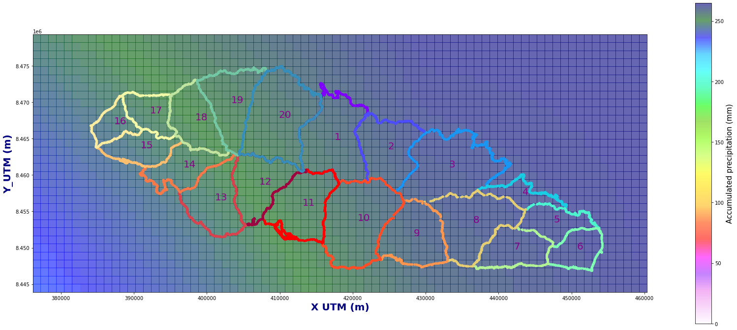
Rain in the different basins#
For each of the different basins, the rainfall has been downscaled and averaged in order to include an spatial rainfall constant throughout the basin.
x_utm, y_utm = tc_total_rain_site(tc, dss_area, figsize=[25,12], basins=basins)#, vmax=970)
dss_area['X_UTM'] = (('lon'), x_utm)
dss_area['Y_UTM'] = (('lat'), y_utm)
dss_area
<xarray.Dataset>
Dimensions:      (lat: 32, lon: 78)
Coordinates:
  * lon          (lon) float64 187.9 187.9 187.9 187.9 ... 188.6 188.6 188.6
  * lat          (lat) float64 -14.07 -14.06 -14.05 ... -13.78 -13.77 -13.76
Data variables:
    rain         (lat, lon) float64 232.9 233.4 233.9 ... 264.7 264.7 264.7
    cell_counts  (lat, lon) float64 1.105e+04 1.112e+04 ... 1.672e+04 1.673e+04
    X_UTM        (lon) float64 3.767e+05 3.778e+05 ... 4.588e+05 4.598e+05
Y_UTM (lat) float64 8.444e+06 8.446e+06 ... 8.478e+06 8.479e+06- lat: 32
- lon: 78
- lon(lon)float64187.9 187.9 187.9 ... 188.6 188.6
array([187.858, 187.868, 187.878, 187.888, 187.898, 187.908, 187.918, 187.928, 187.938, 187.948, 187.958, 187.968, 187.978, 187.988, 187.998, 188.008, 188.018, 188.028, 188.038, 188.048, 188.058, 188.068, 188.078, 188.088, 188.098, 188.108, 188.118, 188.128, 188.138, 188.148, 188.158, 188.168, 188.178, 188.188, 188.198, 188.208, 188.218, 188.228, 188.238, 188.248, 188.258, 188.268, 188.278, 188.288, 188.298, 188.308, 188.318, 188.328, 188.338, 188.348, 188.358, 188.368, 188.378, 188.388, 188.398, 188.408, 188.418, 188.428, 188.438, 188.448, 188.458, 188.468, 188.478, 188.488, 188.498, 188.508, 188.518, 188.528, 188.538, 188.548, 188.558, 188.568, 188.578, 188.588, 188.598, 188.608, 188.618, 188.628]) - lat(lat)float64-14.07 -14.06 ... -13.77 -13.76
array([-14.068, -14.058, -14.048, -14.038, -14.028, -14.018, -14.008, -13.998,
       -13.988, -13.978, -13.968, -13.958, -13.948, -13.938, -13.928, -13.918,
       -13.908, -13.898, -13.888, -13.878, -13.868, -13.858, -13.848, -13.838,
       -13.828, -13.818, -13.808, -13.798, -13.788, -13.778, -13.768, -13.758])
- rain(lat, lon)float64232.9 233.4 233.9 ... 264.7 264.7
array([[232.87567292, 233.39373645, 233.91179999, ..., 263.34440372, 263.53992748, 263.73545124], [233.35072892, 233.86316845, 234.37560797, ..., 263.38829996, 263.57783974, 263.76737952], [233.82578492, 234.33260044, 234.83941595, ..., 263.4321962 , 263.615752 , 263.79930781], ..., [246.65229689, 247.0072642 , 247.36223152, ..., 264.61739465, 264.63938308, 264.66137152], [247.12735289, 247.4766962 , 247.8260395 , ..., 264.66129089, 264.67729535, 264.6932998 ], [247.60240889, 247.94612819, 248.28984749, ..., 264.70518713, 264.71520761, 264.72522809]]) - cell_counts(lat, lon)float641.105e+04 1.112e+04 ... 1.673e+04
array([[11047.73039999, 11115.66079999, 11183.59119999, ..., 17324.07519998, 17437.45039998, 17550.82559998], [11141.45079999, 11208.80159999, 11276.15239999, ..., 17304.25039998, 17414.35079998, 17524.45119998], [11235.17119999, 11301.94239999, 11368.71359999, ..., 17284.42559998, 17391.25119998, 17498.07679998], ..., [13765.62199999, 13816.74399999, 13867.86599999, ..., 16749.156 , 16767.562 , 16785.968 ], [13859.34239999, 13909.88479999, 13960.42719999, ..., 16729.3312 , 16744.4624 , 16759.5936 ], [13953.06279999, 14003.02559999, 14052.98839999, ..., 16709.5064 , 16721.3628 , 16733.2192 ]]) - X_UTM(lon)float643.767e+05 3.778e+05 ... 4.598e+05
array([376703.63267878, 377783.41091207, 378863.18583949, 379942.95749027, 381022.72589363, 382102.49107878, 383182.25307494, 384262.01191132, 385341.76761715, 386421.52022164, 387501.26975401, 388581.01624346, 389660.75971922, 390740.50021051, 391820.23774652, 392899.97235649, 393979.70406962, 395059.43291512, 396139.15892221, 397218.88212011, 398298.60253802, 399378.32020515, 400458.03515072, 401537.74740394, 402617.45699401, 403697.16395016, 404776.86830159, 405856.5700775 , 406936.26930712, 408015.96601965, 409095.66024429, 410175.35201027, 411255.04134678, 412334.72828303, 413414.41284823, 414494.0950716 , 415573.77498233, 416653.45260963, 417733.12798272, 418812.80113079, 419892.47208305, 420972.14086872, 422051.80751699, 423131.47205707, 424211.13451817, 425290.79492949, 426370.45332023, 427450.10971961, 428529.76415682, 429609.41666106, 430689.06726155, 431768.71598749, 432848.36286808, 433928.00793251, 435007.65121001, 436087.29272976, 437166.93252097, 438246.57061284, 439326.20703458, 440405.84181539, 441485.47498446, 442565.10657101, 443644.73660422, 444724.36511331, 445803.99212747, 446883.61767591, 447963.24178782, 449042.8644924 , 450122.48581886, 451202.1057964 , 452281.72445421, 453361.3418215 , 454440.95792746, 455520.57280129, 456600.1864722 , 457679.79896938, 458759.41032203, 459839.02055935]) - Y_UTM(lat)float648.444e+06 8.446e+06 ... 8.479e+06
array([8444454.50439584, 8445560.65557849, 8446666.80588357,
       8447772.95531166, 8448879.10386332, 8449985.25153914,
       8451091.39833969, 8452197.54426554, 8453303.68931727,
       8454409.83349545, 8455515.97680067, 8456622.11923348,
       8457728.26079448, 8458834.40148423, 8459940.54130332,
       8461046.68025231, 8462152.81833178, 8463258.95554231,
       8464365.09188448, 8465471.22735886, 8466577.36196603,
       8467683.49570657, 8468789.62858104, 8469895.76059004,
       8471001.89173412, 8472108.02201388, 8473214.15142989,
       8474320.27998272, 8475426.40767295, 8476532.53450117,
       8477638.66046794, 8478744.78557385])
x_utm, y_utm, INFO = tc_total_rain_site(tc, dss_area, figsize=[25,12], rain=0, basins=basins, points=1)#, vmax=970)
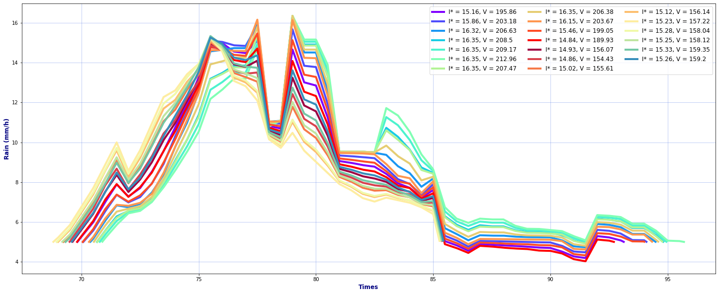
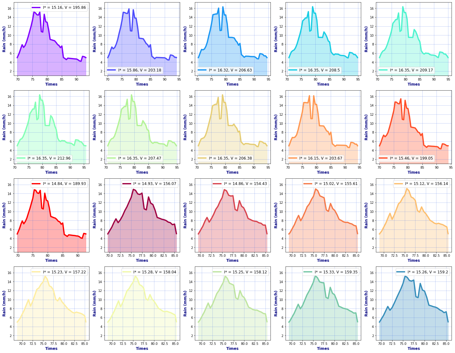
Hyetograph for each basin#
The rainfall over time has been then obtained for each of the following basins, as it will be the input of the flooding model.
D_5 = Plot_Rain_Hyetograph_Basins(dst_area, dss_area, basins, INFO, site, thr_plot=1, thr=5)
D_5.to_netcdf(os.path.join(p_deliv, 'Rain_Real_Basins_' + site + '_Tc_' + str(tc.name.values) + '_sp' + str(n) + '.nc'))