Flooding Model

import warnings
warnings.filterwarnings('ignore')

import os
import os.path as op
import sys
import glob

import matplotlib.pyplot as plt
import xarray as xr
import pandas as pd
import numpy as np
import matplotlib.patches as patches
import matplotlib
import geopandas as gpd

sys.path.insert(0, op.join(op.abspath(''), '..','..',  '..'))

from bluemath.rainfall_forecast.rainfall_forecast import *

Warning: cannot import cf-json, install "metocean" dependencies for full functionality

# database
p_data = r'/media/administrador/HD2/SamoaTonga/data'
site, site_, nm = 'Savaii', 'savaii', 'sp'
p_site = op.join(p_data, site)

p_deliv = op.join(p_site, 'd09_rainfall_forecast')

#Basins path
p_basins = op.join(p_deliv, 'basins', nm + '_db' +  '_fixed.shp')

#Historical TC example
tc='amos'

#Dem
p_dem = os.path.join(p_deliv, site_ + '_5m_dem.nc')

#output files
p_flood_real_nc = os.path.join(p_deliv,  'Flooding_Real_' + tc + '_' + nm + '_xyz_points.nc')
p_flood_real_txt = os.path.join(p_deliv, 'Flooding_Real_' + tc + '_' + nm + '_xyz_points.txt')

run=False #Run flooding extraction

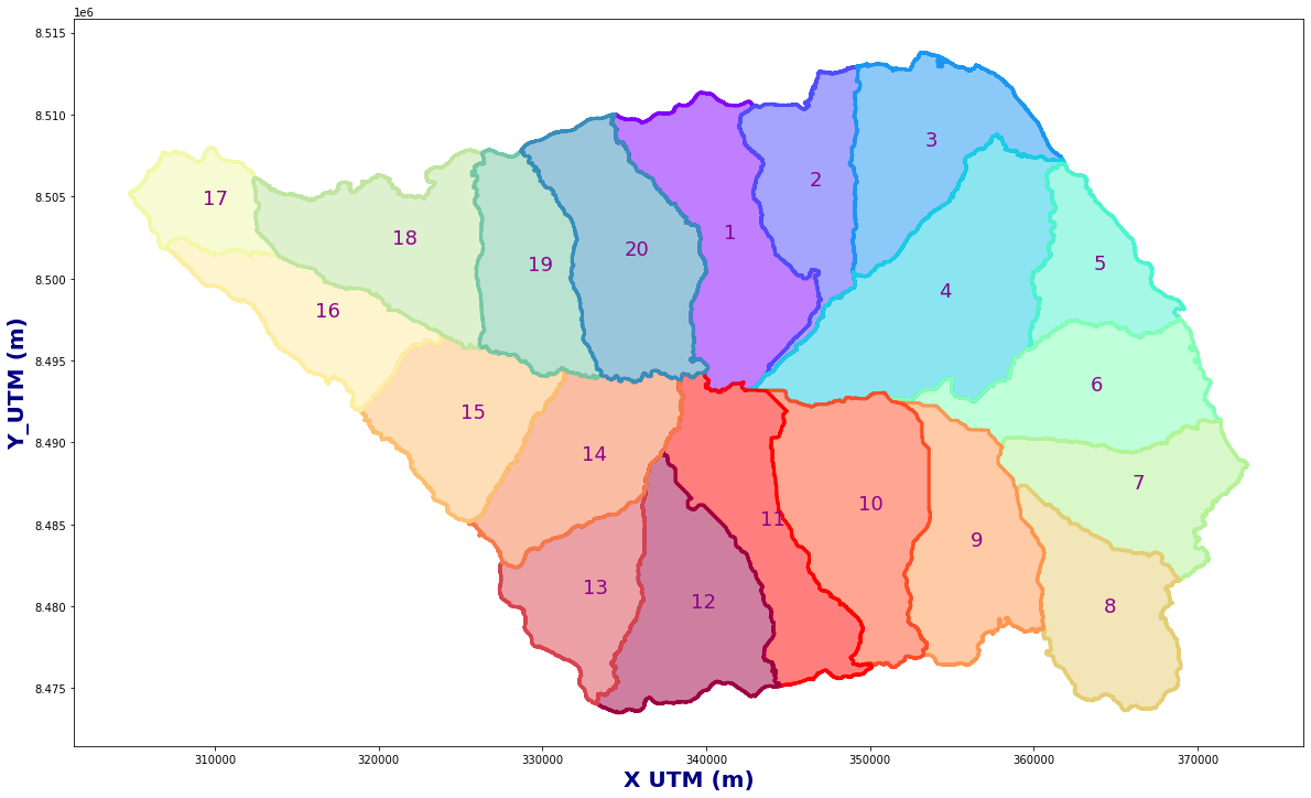
Basins

#Basins
bas_raw = gpd.read_file(p_basins)
basins = Obtain_Basins(bas_raw, site)
Plot_Basins(basins)

dem = xr.open_dataset(p_dem).rename({'z':'elevation'})
res_f = 4; dem=dem.isel(x=np.arange(0, len(dem.x.values),res_f), y = np.arange(0, len(dem.y.values),res_f))
dem['elevation'] = (('y', 'x'), np.where(dem.elevation.values < 0, np.nan, dem.elevation.values))
dem

<xarray.Dataset>
Dimensions:    (x: 3751, y: 2351)
Coordinates:
  * x          (x) float64 3.03e+05 3.03e+05 3.03e+05 ... 3.78e+05 3.78e+05
  * y          (y) float64 8.469e+06 8.469e+06 8.469e+06 ... 8.516e+06 8.516e+06
Data variables:
    elevation  (y, x) float32 nan nan nan nan nan nan ... nan nan nan nan nan
Attributes:
    description:  EPSG:32702

Flooding

For the different basins, and after simulating the hydrographs, below are the results of the flooding extents

run = True

if run:
    OUT = Get_Flood_All_Basins_real(basins, p_deliv, site_, nm, tc, thr=0.05)
    OUT.to_xarray().rename({'index':'point'}).to_netcdf(p_flood_real_nc)
    np.savetxt(p_flood_real_txt, OUT.values)
    OUT = xr.open_dataset(p_flood_real_nc).to_dataframe()
else:
    OUT = xr.open_dataset(p_flood_real_nc).to_dataframe()

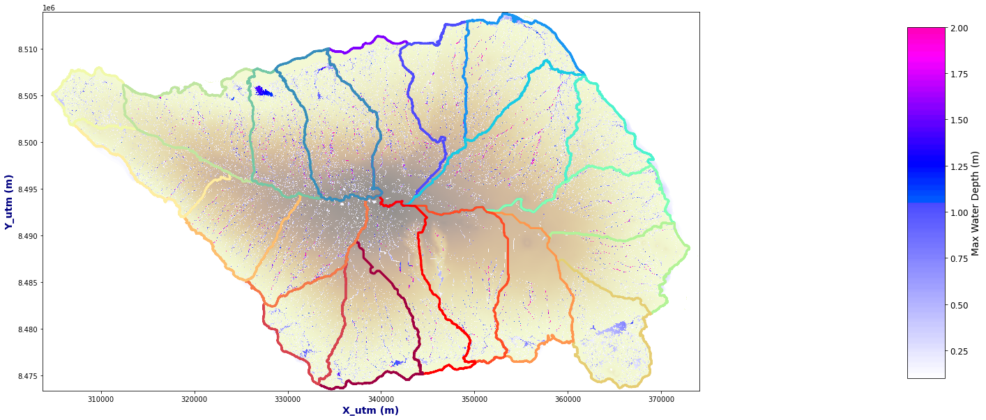
Regional Scale

From the rainfall hydrographs obtained in the previous section, LISFLOOD-FP model has been used to obtain the flooding extents. LISFLOOD-FP is a two-dimensional hydrodynamic model developed by the University of Bristol. The model is specifically designed to simulate floodplain inundation in a computationally efficient manner over complex topography. It predicts water depths in each grid cell at each time step, and hence can simulate the dynamic propagation of flood waves over fluvial, coastal and estuarine floodplains.

LISFLOOD-FP set up for each drainage basin has been carefully made taking into consideration the boundary conditions, the friction model (Manning’s n friction coefficients obtained from land use data), the total simulation time so the time of maximum inundation is being captured, the best execution mode for the model and the optimal values of the hydraulic parameters.

Plot_Rain_Basins(basins, p_deliv, site_, nm = nm, tc=tc, d_min=0.1, dem=dem)

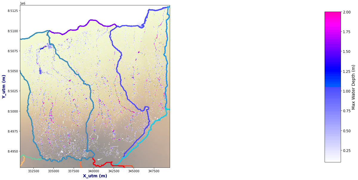
Basin Scale

Plot_Rain_Basins(basins, p_deliv, site_,  nm, tc, dem=dem,d_min=.1, basins_sel=[0,1,19])