Flooding Metamodel

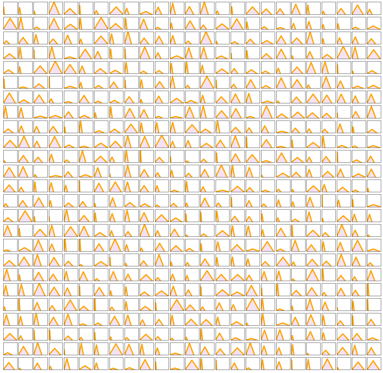
The storms, which are the rainfall input for LISFLOOD-FP model, have been defined as triangles. Each triangle shaped storm has its corresponding duration D in hours, peak intensity Z* in millimeters per hour and rainfall volume V (area under the triangle) in mm3/mm2. From the developed TC rain model it is known that the peak intensity goes up to 50 mm/hr, and a threshold of 4 mm/hr is set as a significant rainfall to be considered. For the duration storms from 1 to 24 hours have been considered.

Latin Hipercube + MDA

A selection of cases based on these ranges of values that the two variables can achieve has been done through a sampling algorithm, Latin Hypercube Sampling (LHS) and a selection algorithm, Maximum Dissimilarity Algorithm (MDA).

import os
import os.path as op
import sys
import warnings
warnings.filterwarnings('ignore')

from scipy.stats import qmc
import pandas as pd
import numpy as np
from sklearn.cluster import KMeans

sys.path.insert(0, op.join(op.abspath(''), '..', '..', '..'))

from bluemath.teslakit.mda import MaxDiss_Simplified_NoThreshold  #We add teslakit path to path manager
from bluemath.rainfall_forecast.LHS import *
from bluemath.rainfall_forecast.rainfall_forecast import *
from bluemath.rainfall_forecast.graffiti_rain import *

Warning: cannot import cf-json, install "metocean" dependencies for full functionality

# database
p_data = r'/media/administrador/HD2/SamoaTonga/data'
site, site_, nm = 'Savaii', 'savaii', 'sp'
p_site = op.join(p_data, site)

p_deliv = op.join(p_site, 'd09_rainfall_forecast')

#Basins path
p_basins = op.join(p_deliv, 'basins', nm + '_db' +  '_fixed.shp')

#Historical TC example
tc, n = 'amos', 166
p_hist_track = os.path.join(p_deliv,'sp_{0}.nc'.format(n))
times_sel = [150, 385] #Times to cut that specific track to our area
p_rain_out = os.path.join(p_deliv,'rain_sp_{0}.nc'.format(n))

#Dem
p_dem = os.path.join(p_deliv, site_ + '_5m_dem.nc')

#Lisflood database

p_lf_db = r'/media/administrador/HD1/DATABASES/Lisflood_Rainfall'

#output files

p_lhs_dataset = os.path.join(p_deliv, 'LHS_dataset_lisflood_rain.nc')
p_lhs_subset = os.path.join(p_deliv, 'LHS_mda_sel_lisflood_volume_rain.nc')

p_mmdl_tc = os.path.join(p_deliv,  'Flooding_Metamodel_Analogues_' + tc + '_' + nm + '_xyz_points.txt')
p_mmdl_tc_nc = os.path.join(p_deliv, 'Flooding_Metamodel_Analogues_' + tc + '_' + nm + '_xyz_points.nc')

p_mmdl_tc

'/media/administrador/HD2/SamoaTonga/data/Savaii/d09_rainfall_forecast/Flooding_Metamodel_Analogues_amos_sp_xyz_points.txt'

#Basins
bas_raw = gpd.read_file(p_basins)
basins = Obtain_Basins(bas_raw, site)

LHS

LHS cuts each dimension space, (Intensity, I* or duration, D, in this case) into n (10 000) sections, where n is the number of sampling points, and only one combination in each section is kept. It produces samples that reflect the true underlying distribution, and it tends to require much smaller sample sizes than simple random sampling.

n_dims = 2 #Number of dimensions
name_dims=['D', 'I*']
n_dims = len(name_dims); #2 #Number of dimensions

lower_bounds = [1, 5] 
upper_bounds = [24 ,50]
n_samples=10000 #Number of combinations to extract from LHS

sampler = qmc.LatinHypercube(d=n_dims, seed=0)
dataset = sampler.random(n=n_samples)
dataset = qmc.scale(dataset, lower_bounds, upper_bounds)

VT = Calculate_Volume_Hydrograph(dataset)
DATASET = pd.DataFrame(dataset, columns=name_dims).to_xarray()
DATASET['V'] = (('index'), VT)
DATASET.to_netcdf(p_lhs_dataset)

Volumes range from 2.79 to 598.91

num=625 #First num cases
Plot_Volume_hidrographs_rain(dataset, num, labels=False)

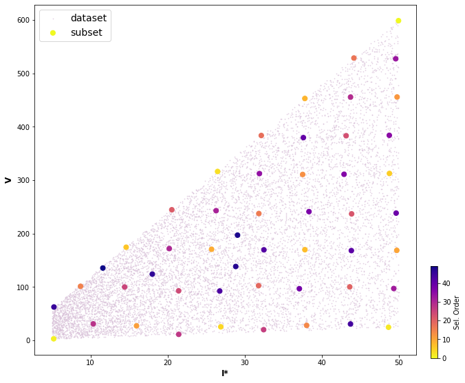
MDA

Then I* and V variables are chosen to apply MDA, with the aim of selecting a representative subset of m cases (50) which best captures the variability of the space.

dataset_mda_v = np.vstack([DATASET['V'].values,DATASET['I*'].values]).T

name_dims_mda_v=['V', 'I*']
n_subset = 200 #Subset for MDA
ix_scalar = [0,1]
ix_directional = []

subset_mda_v = MaxDiss_Simplified_NoThreshold(dataset_mda_v, n_subset, ix_scalar, ix_directional)
df_v = pd.DataFrame(subset_mda_v, columns=name_dims_mda_v).to_xarray()

D=[]
for i in df_v.index.values:
    D.append(DATASET['D'].values[np.where((np.round(DATASET['V'].values,8)==np.round(df_v['V'][i].values,8)) & (np.round(DATASET['I*'].values,8)==np.round(df_v['I*'][i].values,8)))[0]][0])
df_v['D']=(('index'), np.array(D))
df_v.to_netcdf(p_lhs_subset)

MaxDiss waves parameters: 10000 --> 200

   MDA centroids: 200/200

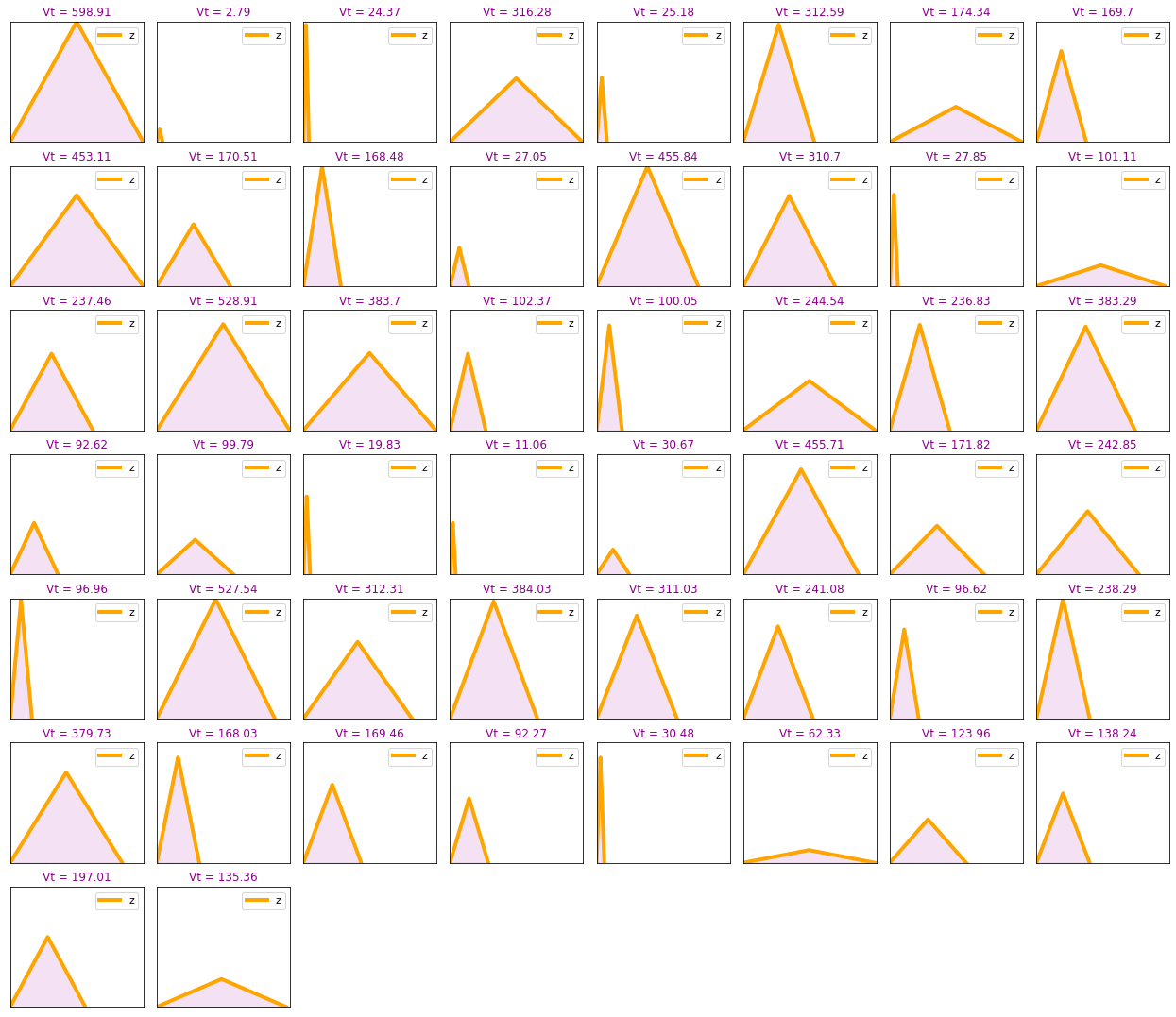
n_cases = 50 #Number of cases selected for lisflood

df_v = df_v.isel(index=range(n_cases))
Plot_MDA_Data(pd.DataFrame(dataset_mda_v), pd.DataFrame(subset_mda_v[:n_cases,:]), d_lab=name_dims_mda_v, figsize=[10,8], s_mda=200)

plt_h = np.vstack([df_v['D'].values,df_v['I*'].values]).T
Plot_Volume_hidrographs_rain(plt_h, n_cases)

Lisflood Simulations

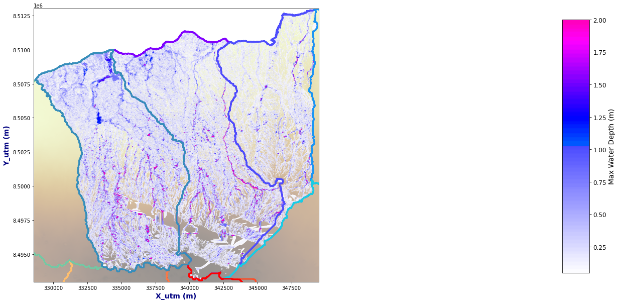
The 50 output simulations from Lisflood for the defined hydrographs above, is presented for one specific basin in he plots below.

bn=1 #Basin to plot (Starting in 1)

bn_out = xr.open_dataset(op.join(p_lf_db, 'Lisflood_' + nm + '_basin_' + str(bn) + '.nc'))

fig = plt.figure(figsize=[20,25])
gs=gridspec.GridSpec(8,8, hspace=0.1, wspace=0.05)

for c in range(n_cases):
    
    try:
        ax=fig.add_subplot(gs[c])
        Plot_Rain_Basins(basins, p_deliv,  site, nm, tc=[], tcs=False, labels=False, out=bn_out.sel(case=c+1), basins_sel=[bn-1],fig=fig, ax=ax)
    except:
        print('Not case: ' + str(c))

TC

tco = xr.open_dataset(p_hist_track)
tc = process_tc_file(tco)
#We can select the dates we are interested in
tc = tc.isel(date_time=slice(times_sel[0], times_sel[1]))
fig_tc = Plot_track(tc, figsize=[20,10], cmap='jet_r', m_size=10)

TC: AMOS, starting day 2016-04-17

Analogue

For a particular TC, the total rainfall footprint of the TC is first obtained through the previously explained TC rain model. Then, the rainfall time series through the basin of interest is extracted. For this rainfall profile the three most similar storms are sought amongst the 50 cases simulated and the flooding map is obtained from the three maps of these three cases through weighted average based on their similarity (closeness) to the actual case.

subset_norm = np.vstack([(df_v['V'].values-np.nanmean(df_v['V'].values))/np.std(df_v['V'].values),
           (df_v['I*'].values-np.nanmean(df_v['I*'].values))/np.std(df_v['I*'].values)]).T

rain = xr.open_dataset(os.path.join(p_deliv, 'Rain_Real_Basins_' + site + '_Tc_' + str(tc.name.values) + '_sp' + str(n) + '.nc'))

tc_rain_norm = np.vstack([(rain['Volume'].values-np.nanmean(df_v['V'].values))/np.std(df_v['V'].values),
           (rain['I'].values-np.nanmean(df_v['I*'].values))/np.std(df_v['I*'].values)]).T

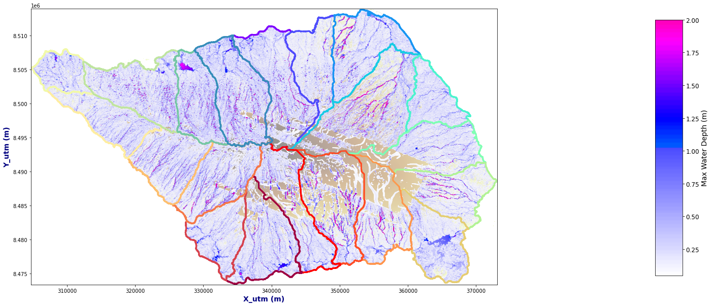
Plot_Basins(basins)
n_an=3 #Number of analogue points
AN = Get_Analogues(n_an, tc_rain_norm, subset_norm, df_v)
AN.to_netcdf(os.path.join(p_deliv, 'Analogues_' + site + '_Tc_' + str(tc.name.values) + '_sp' + str(n) + '.nc'))
Plot_Analogues(df_v, rain, AN, basins)

Historial TC

dem = xr.open_dataset(p_dem).rename({'z':'elevation'})
res_f = 2; dem=dem.isel(x=np.arange(0, len(dem.x.values),res_f), y = np.arange(0, len(dem.y.values),res_f))
dem['elevation'] = (('y', 'x'), np.where(dem.elevation.values < 0, np.nan, dem.elevation.values))

OUT = Get_Flood_All_Basins(basins, AN, p_lf_db, nm)
np.savetxt(p_mmdl_tc, OUT.values)
OUT.to_xarray().rename({'index':'point'}).to_netcdf(p_mmdl_tc_nc)
Plot_Rain_Flood_Points(basins, OUT, dem=dem)

Basin 20

OUT = Get_Flood_All_Basins(basins, AN, p_lf_db, nm, basins_sel=[0, 1, 19])
Plot_Rain_Flood_Points(basins, OUT, dem=dem)

Basin 20