Historical TC : Evan (2012)
Contents
Historical TC : Evan (2012)#
# common
import os
import os.path as op
import sys

# pip
import numpy as np
import xarray as xr
import wavespectra

# DEV: bluemath
sys.path.insert(0, op.join(op.abspath(''), '..', '..', '..', '..'))

# bluemath modules
from bluemath.greensurgerepo.storms import historic_track_preprocessing, historic_track_interpolation, get_category
from bluemath.greensurgerepo.vortex import vortex_model_general
from bluemath.greensurgerepo.greensurge import GS_wind_partition, print_GFD_properties, GS_windsetup_reconstruction, presure_to_IB

from bluemath.binwaves.forecast import cut_resample_area, reconstruct_spec

from bluemath.greensurgerepo.plots.plots_greensurge import plot_case_input, plot_presure_vs_IB

from bluemath.astronomical_tide import calculate_AT_TPXO9v4

from bluemath.wswan.plots.common import custom_cmap, bathy_cmap

from bluemath.tc_forecast import Plot_Swath_ShyTCWaves, Plot_Swath_ShyTCWaves_coords, \
Plot_SuperPoint_TC_Forecast, Plot_Grid_HsTmDp, Plot_Grid_TWL_max, Plot_Grid_SWATH, \
Plot_TWL_timeseries, Plot_Grid_HsPd_series
from bluemath.tc_forecast import animate_tc_hs_ss_tide_twl_forecast

# hide warnings
import warnings
warnings.filterwarnings('ignore')
## Methodology
BinWaves
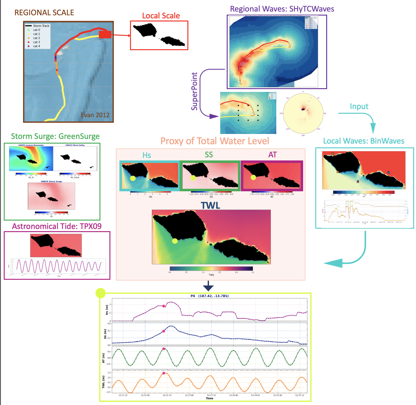
In this section we will make use of the combination of SHyTCWaves and Greensurge at a regional scale, and BinWaves at a local scale, to obtain the evolution of waves and water levels caused by TC Evan in 2012
Database and site parameters#
p_data = r'/media/administrador/HD2/SamoaTonga/data'
site = 'Samoa'
p_site = op.join(p_data)

#path databases
p_db = r'/media/administrador/HD1/DATABASES'

# deliverable folder
p_deliv = op.join(p_site, 'd06_tc_inundation_forecast')

# historical TCs (ibtracs)
p_ibtracs = op.join(p_deliv, 'IBTrACS.ALL.v04r00.nc')

# tc forecast
p_tcforecast = op.join(p_deliv, 'TC_forecast')

# ShyTCWaves
p_shy_grid = os.path.join(p_tcforecast, 'Super_Points', 'xds_shy_bulk_Samoa_EVAN_2012.nc')
p_superpoint_shytcwaves = os.path.join(p_tcforecast, 'Super_Points', 'xds_shy_sp_Samoa_EVAN_2012.nc')

# BinWaves: superpoint and reconstruction coefficients
deg_sup = 15
area_extraction =  [-172.85+360, -171.38+360, -14.09, -13.41]
resample_factor = 10

p_deliv_d05 = op.join(p_site, 'd05_swell_inundation_forecast')
p_superpoint_binwaves = op.join(p_deliv_d05, 'spec', 'super_point_superposition_{0}_.nc'.format(deg_sup))
p_swan_output = op.join(p_deliv_d05, 'swan', 'binwaves', 'out_main_binwaves.nc')
p_kp_coeffs = op.join(p_deliv_d05, 'reconstruction', 'kp_grid')

# GreenSurge
domain_study='Samoa'
p_greensurge = op.join(p_db, 'greensurge')
p_GFD_libdir = op.join(p_greensurge, 'GFD_lib', site, 'GFD_Samoa_T84_W40_D15_24h_CDdefault')
p_GFD_info = op.join(p_GFD_libdir, 'GFD_lib_info.nc')

# astronomical tide
model_directory = op.join(p_db, 'TPX09_atlas_v4')


# model execution parameters
run_binwaves = False
run_green_WS = True
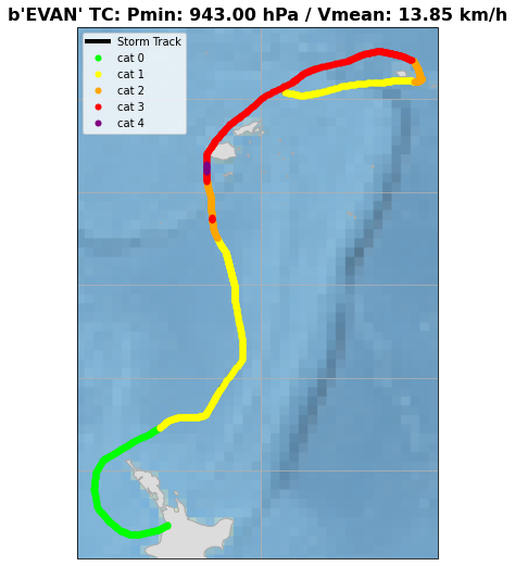
TC Selection#
With the name and the year we can select here any historical TC from IBTrACS
ibtracs = xr.open_dataset(p_ibtracs)

name = b'EVAN'
year = 2012
centerID = 'WMO'

storm = ibtracs.isel(
    storm = np.where(
        (ibtracs.name == name) & \
        (ibtracs.time[:,0].dt.year.values == year)
    )[0]
).isel(storm=0)
# preprocess selected historic TC: obtain strom variables
df_TC_hist = historic_track_preprocessing(storm, center = centerID)

# computational time step mandatory for GS methodology:
dt_comp = 20  # minutes

# generate interpolated storm track and mandatory data to apply vortex model
storm_track, time_input = historic_track_interpolation(df_TC_hist, dt_comp)
plot_case_input(storm_track, name);
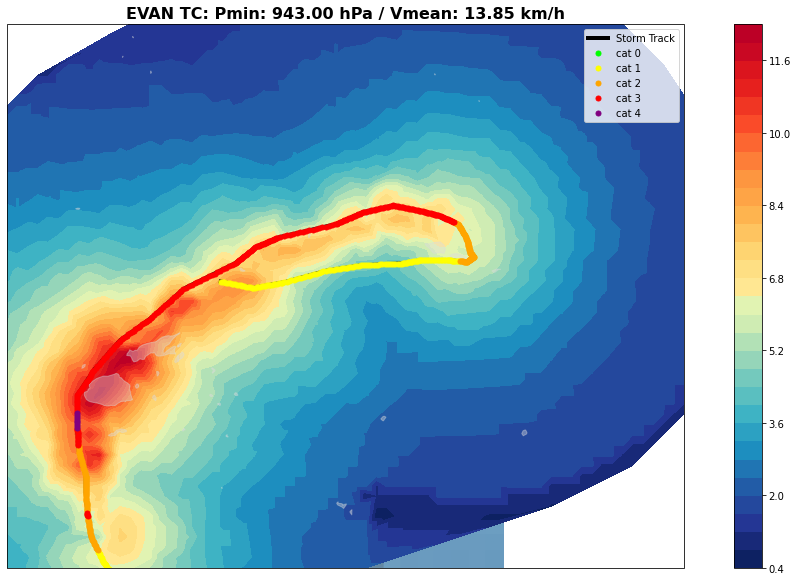
ShyTCWaves#
SHyTCWaves
Using SHyTCWaves we are able of obtaining the SWATH for the wave parameters and the evolution of the SuperPoint directional spectra over time.
SWATH#
TC_grid = xr.open_dataset(p_shy_grid)
Plot_Swath_ShyTCWaves(
    TC_grid, storm_track,
    name,
    var = 'hswath',
    cmap = custom_cmap(50, 'YlOrRd', 0.15, 0.9, 'YlGnBu_r', 0, 0.85),
);
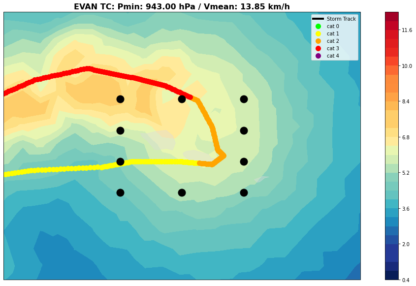
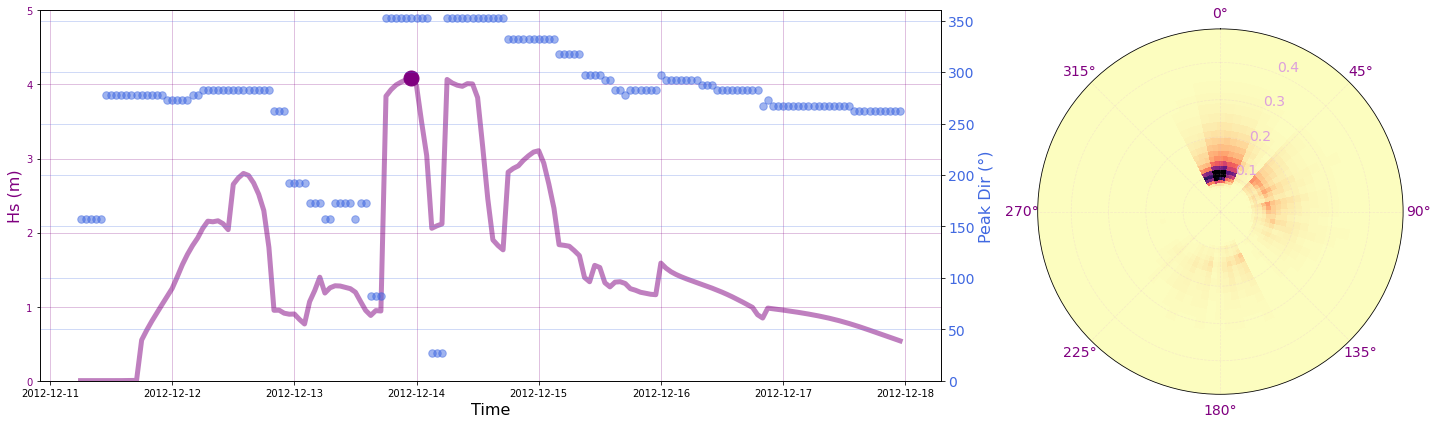
SuperPoint#
Locations od the SuperPoint surrounding our study site
sp = xr.open_dataset(p_superpoint_shytcwaves)

Plot_Swath_ShyTCWaves_coords(
    TC_grid, storm_track,
    name,
    sp,
    mksize = 20,
    var = 'hswath',
    cmap = custom_cmap(15, 'YlOrRd', 0.15, 0.9, 'YlGnBu_r', 0, 0.85),
);
time_s = sp.time[np.nanargmax(sp.efth.spec.hs().values)]

Plot_SuperPoint_TC_Forecast(sp, time_s, ymax=5, figsize=[20,6]);
BinWaves#
BinWaves
Using the SuperPoint information from SHyTCWaves at a regional scale, we downscale the waves locally my means of BinWaves1.
out_sim_swan = xr.open_dataset(p_swan_output)

out_sim = cut_resample_area(
    out_sim_swan, area_extraction,
    resample_factor,
    case = 15,
    plot = False,
)
We interpolate the spectra to the same coordinates used to run BinWaves
coords_binwaves = xr.open_dataset(p_superpoint_binwaves).isel(time=0)

sp = sp.interp(
    dir = coords_binwaves.dir.values,
    freq = coords_binwaves.freq.values,
)
# binwaves spec reconstruction
name_recon = 'binwaves_{0}_{1}.nc'.format(name.decode("utf-8"), year)
p_recon = op.join(p_tcforecast, name_recon)

if run_binwaves:
    sp_p = reconstruct_spec(p_kp_coeffs, sp, out_sim)
    sp_p.to_netcdf(p_recon)

else:
    sp_p = xr.open_dataset(p_recon)
Generating nearshore forecast...: 100%|██████████████████████████████| 1127/1127
# use wavespectra to calculate Hs, Tp, Tm and Dp
sp_p['Hs'] = sp_p.efth.spec.hs()
sp_p['Tp'] = sp_p.efth.spec.tp()
sp_p['Tm'] = sp_p.efth.spec.tm02()
sp_p['Dp'] = sp_p.efth.spec.dp()
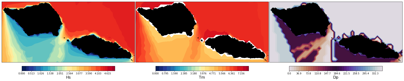
Below are the maps for the time in which the SuperPoint energy was the highest
Plot_Grid_HsTmDp(sp_p, time_s);
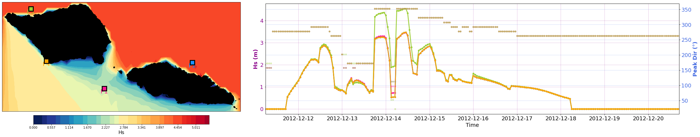
SWATH#
Here we define a list of interest points to see the evolution of the wave height and direction over time
points_interest = np.array([
    [-172.23,-171.699, -172.675,-172.58],
    [-13.95, -13.794 , -13.47, -13.785],
])

points_names = ['P1', 'P2', 'P3', 'P4' ]
Plot_Grid_HsPd_series(sp, sp_p, points_interest, p_kp_coeffs, out_sim, points_names);
Generating nearshore forecast...: 100%|██████████████████████████████| 1/1 [00:0
Generating nearshore forecast...: 100%|██████████████████████████████| 1/1 [00:0
Generating nearshore forecast...: 100%|██████████████████████████████| 1/1 [00:0
Generating nearshore forecast...: 100%|██████████████████████████████| 1/1 [00:0
GreenSurge#
p_GFD_info = op.join(p_GFD_libdir, 'GFD_lib_info.nc')
ds_GFD_info = xr.open_dataset(p_GFD_info)

print_GFD_properties(ds_GFD_info, domain_study)
GFD info:
---------
Samoa domain
84 cells, 29*25 km resolution
24 wind directions, 15º resolution
Unit wind speed: 40m/s
CD formulation: Wu1982
tini = np.datetime64('2012-12-11T00:00')
tend = np.datetime64('2012-12-15T17:00')

storm_track_sel = storm_track[(storm_track.index >= tini) & (storm_track.index <= tend)]

xds_vortex_GS = vortex_model_general(storm_track_sel, ds_GFD_info)
# TODO reactivar
ds_wind_partition = GS_wind_partition(ds_GFD_info, xds_vortex_GS)
Run: Searching for analogues, re-scaling and applying wind-drag coefficient
# TODO reactivar
ds_WL_GS_WindSetUp = GS_windsetup_reconstruction(
    p_GFD_libdir, ds_GFD_info,
    ds_wind_partition, xds_vortex_GS,
)
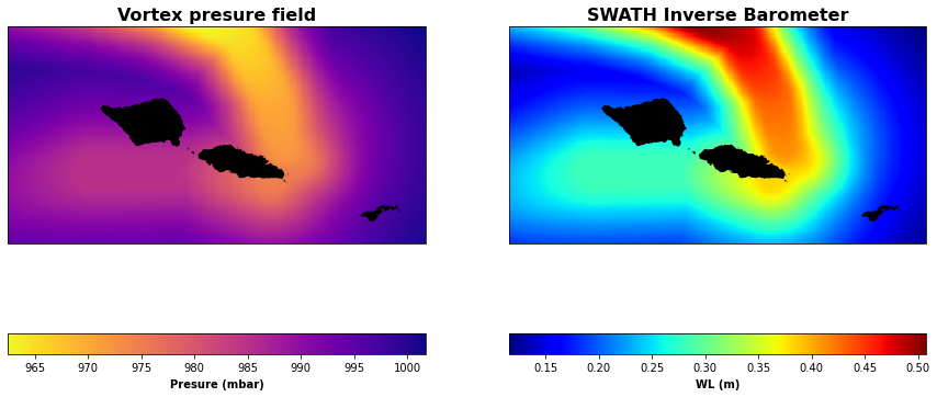
ds_WL_GS_IB = presure_to_IB(xds_vortex_GS)
plot_presure_vs_IB(
    xds_vortex_GS, ds_WL_GS_IB, storm_track,
    swath = True,
    figsize = [15,15],
);
# Prepare TWL dataset

u = np.intersect1d(sp_p.time.values, ds_WL_GS_WindSetUp.time.values)
sp_p = sp_p.sel(time = u).get(['Hs', 'Tp', 'Dp'])
ds_WL_GS_WindSetUp = ds_WL_GS_WindSetUp.sel(time = u)

TWL = sp_p.interp(
    lon = ds_WL_GS_WindSetUp.lon.values,
    lat = ds_WL_GS_WindSetUp.lat.values,
).transpose('time','lon','lat')

ds_WL_GS_IB = ds_WL_GS_IB.interp(
    lon = ds_WL_GS_WindSetUp.lon.values,
    lat = ds_WL_GS_WindSetUp.lat.values,
)

TWL['WL_IB'] = (('time','lon','lat'), ds_WL_GS_IB.resample(time='1h').max().sel(time=u).transpose('time','lon','lat').WL.values)
TWL['WL_SetUp'] = (('time','lon','lat'), ds_WL_GS_WindSetUp.WL.values)
TWL['SS'] = TWL['WL_SetUp'] + TWL['WL_IB']

TWL
<xarray.Dataset>
Dimensions:   (lat: 365, lon: 654, time: 107)
Coordinates:
  * time      (time) datetime64[ns] 2012-12-11T06:00:00 ... 2012-12-15T16:00:00
  * lon       (lon) float64 186.7 186.7 186.7 186.7 ... 189.6 189.6 189.6 189.6
  * lat       (lat) float64 -14.54 -14.54 -14.53 -14.53 ... -12.91 -12.91 -12.9
Data variables:
    Hs        (time, lon, lat) float64 nan nan nan nan nan ... nan nan nan nan
    Tp        (time, lon, lat) float64 nan nan nan nan nan ... nan nan nan nan
    Dp        (time, lon, lat) float64 nan nan nan nan nan ... nan nan nan nan
    WL_IB     (time, lon, lat) float64 nan 0.03122 0.03122 ... 0.009899 0.009898
    WL_SetUp  (time, lon, lat) float64 0.0 4.728e-06 ... 8.177e-05 8.631e-05
SS (time, lon, lat) float64 nan 0.03123 0.03122 ... 0.009981 0.009985- lat: 365
- lon: 654
- time: 107
- time(time)datetime64[ns]2012-12-11T06:00:00 ... 2012-12-...
array(['2012-12-11T06:00:00.000000000', '2012-12-11T07:00:00.000000000', '2012-12-11T08:00:00.000000000', '2012-12-11T09:00:00.000000000', '2012-12-11T10:00:00.000000000', '2012-12-11T11:00:00.000000000', '2012-12-11T12:00:00.000000000', '2012-12-11T13:00:00.000000000', '2012-12-11T14:00:00.000000000', '2012-12-11T15:00:00.000000000', '2012-12-11T16:00:00.000000000', '2012-12-11T17:00:00.000000000', '2012-12-11T18:00:00.000000000', '2012-12-11T19:00:00.000000000', '2012-12-11T20:00:00.000000000', '2012-12-11T21:00:00.000000000', '2012-12-11T22:00:00.000000000', '2012-12-11T23:00:00.000000000', '2012-12-12T00:00:00.000000000', '2012-12-12T01:00:00.000000000', '2012-12-12T02:00:00.000000000', '2012-12-12T03:00:00.000000000', '2012-12-12T04:00:00.000000000', '2012-12-12T05:00:00.000000000', '2012-12-12T06:00:00.000000000', '2012-12-12T07:00:00.000000000', '2012-12-12T08:00:00.000000000', '2012-12-12T09:00:00.000000000', '2012-12-12T10:00:00.000000000', '2012-12-12T11:00:00.000000000', '2012-12-12T12:00:00.000000000', '2012-12-12T13:00:00.000000000', '2012-12-12T14:00:00.000000000', '2012-12-12T15:00:00.000000000', '2012-12-12T16:00:00.000000000', '2012-12-12T17:00:00.000000000', '2012-12-12T18:00:00.000000000', '2012-12-12T19:00:00.000000000', '2012-12-12T20:00:00.000000000', '2012-12-12T21:00:00.000000000', '2012-12-12T22:00:00.000000000', '2012-12-12T23:00:00.000000000', '2012-12-13T00:00:00.000000000', '2012-12-13T01:00:00.000000000', '2012-12-13T02:00:00.000000000', '2012-12-13T03:00:00.000000000', '2012-12-13T04:00:00.000000000', '2012-12-13T05:00:00.000000000', '2012-12-13T06:00:00.000000000', '2012-12-13T07:00:00.000000000', '2012-12-13T08:00:00.000000000', '2012-12-13T09:00:00.000000000', '2012-12-13T10:00:00.000000000', '2012-12-13T11:00:00.000000000', '2012-12-13T12:00:00.000000000', '2012-12-13T13:00:00.000000000', '2012-12-13T14:00:00.000000000', '2012-12-13T15:00:00.000000000', '2012-12-13T16:00:00.000000000', '2012-12-13T17:00:00.000000000', '2012-12-13T18:00:00.000000000', '2012-12-13T19:00:00.000000000', '2012-12-13T20:00:00.000000000', '2012-12-13T21:00:00.000000000', '2012-12-13T22:00:00.000000000', '2012-12-13T23:00:00.000000000', '2012-12-14T00:00:00.000000000', '2012-12-14T01:00:00.000000000', '2012-12-14T02:00:00.000000000', '2012-12-14T03:00:00.000000000', '2012-12-14T04:00:00.000000000', '2012-12-14T05:00:00.000000000', '2012-12-14T06:00:00.000000000', '2012-12-14T07:00:00.000000000', '2012-12-14T08:00:00.000000000', '2012-12-14T09:00:00.000000000', '2012-12-14T10:00:00.000000000', '2012-12-14T11:00:00.000000000', '2012-12-14T12:00:00.000000000', '2012-12-14T13:00:00.000000000', '2012-12-14T14:00:00.000000000', '2012-12-14T15:00:00.000000000', '2012-12-14T16:00:00.000000000', '2012-12-14T17:00:00.000000000', '2012-12-14T18:00:00.000000000', '2012-12-14T19:00:00.000000000', '2012-12-14T20:00:00.000000000', '2012-12-14T21:00:00.000000000', '2012-12-14T22:00:00.000000000', '2012-12-14T23:00:00.000000000', '2012-12-15T00:00:00.000000000', '2012-12-15T01:00:00.000000000', '2012-12-15T02:00:00.000000000', '2012-12-15T03:00:00.000000000', '2012-12-15T04:00:00.000000000', '2012-12-15T05:00:00.000000000', '2012-12-15T06:00:00.000000000', '2012-12-15T07:00:00.000000000', '2012-12-15T08:00:00.000000000', '2012-12-15T09:00:00.000000000', '2012-12-15T10:00:00.000000000', '2012-12-15T11:00:00.000000000', '2012-12-15T12:00:00.000000000', '2012-12-15T13:00:00.000000000', '2012-12-15T14:00:00.000000000', '2012-12-15T15:00:00.000000000', '2012-12-15T16:00:00.000000000'], dtype='datetime64[ns]') - lon(lon)float64186.7 186.7 186.7 ... 189.6 189.6
array([186.67925, 186.68375, 186.68825, ..., 189.60875, 189.61325, 189.61775])
- lat(lat)float64-14.54 -14.54 ... -12.91 -12.9
array([-14.54225, -14.53775, -14.53325, ..., -12.91325, -12.90875, -12.90425])
- Hs(time, lon, lat)float64nan nan nan nan ... nan nan nan nan
- standard_name :
- sea_surface_wave_significant_height
- units :
- m
array([[[nan, nan, nan, ..., nan, nan, nan], [nan, nan, nan, ..., nan, nan, nan], [nan, nan, nan, ..., nan, nan, nan], ..., [nan, nan, nan, ..., nan, nan, nan], [nan, nan, nan, ..., nan, nan, nan], [nan, nan, nan, ..., nan, nan, nan]], [[nan, nan, nan, ..., nan, nan, nan], [nan, nan, nan, ..., nan, nan, nan], [nan, nan, nan, ..., nan, nan, nan], ..., [nan, nan, nan, ..., nan, nan, nan], [nan, nan, nan, ..., nan, nan, nan], [nan, nan, nan, ..., nan, nan, nan]], [[nan, nan, nan, ..., nan, nan, nan], [nan, nan, nan, ..., nan, nan, nan], [nan, nan, nan, ..., nan, nan, nan], ..., ... ..., [nan, nan, nan, ..., nan, nan, nan], [nan, nan, nan, ..., nan, nan, nan], [nan, nan, nan, ..., nan, nan, nan]], [[nan, nan, nan, ..., nan, nan, nan], [nan, nan, nan, ..., nan, nan, nan], [nan, nan, nan, ..., nan, nan, nan], ..., [nan, nan, nan, ..., nan, nan, nan], [nan, nan, nan, ..., nan, nan, nan], [nan, nan, nan, ..., nan, nan, nan]], [[nan, nan, nan, ..., nan, nan, nan], [nan, nan, nan, ..., nan, nan, nan], [nan, nan, nan, ..., nan, nan, nan], ..., [nan, nan, nan, ..., nan, nan, nan], [nan, nan, nan, ..., nan, nan, nan], [nan, nan, nan, ..., nan, nan, nan]]]) - Tp(time, lon, lat)float64nan nan nan nan ... nan nan nan nan
- standard_name :
- sea_surface_wave_period_at_variance_spectral_density_maximum
- units :
- s
array([[[nan, nan, nan, ..., nan, nan, nan], [nan, nan, nan, ..., nan, nan, nan], [nan, nan, nan, ..., nan, nan, nan], ..., [nan, nan, nan, ..., nan, nan, nan], [nan, nan, nan, ..., nan, nan, nan], [nan, nan, nan, ..., nan, nan, nan]], [[nan, nan, nan, ..., nan, nan, nan], [nan, nan, nan, ..., nan, nan, nan], [nan, nan, nan, ..., nan, nan, nan], ..., [nan, nan, nan, ..., nan, nan, nan], [nan, nan, nan, ..., nan, nan, nan], [nan, nan, nan, ..., nan, nan, nan]], [[nan, nan, nan, ..., nan, nan, nan], [nan, nan, nan, ..., nan, nan, nan], [nan, nan, nan, ..., nan, nan, nan], ..., ... ..., [nan, nan, nan, ..., nan, nan, nan], [nan, nan, nan, ..., nan, nan, nan], [nan, nan, nan, ..., nan, nan, nan]], [[nan, nan, nan, ..., nan, nan, nan], [nan, nan, nan, ..., nan, nan, nan], [nan, nan, nan, ..., nan, nan, nan], ..., [nan, nan, nan, ..., nan, nan, nan], [nan, nan, nan, ..., nan, nan, nan], [nan, nan, nan, ..., nan, nan, nan]], [[nan, nan, nan, ..., nan, nan, nan], [nan, nan, nan, ..., nan, nan, nan], [nan, nan, nan, ..., nan, nan, nan], ..., [nan, nan, nan, ..., nan, nan, nan], [nan, nan, nan, ..., nan, nan, nan], [nan, nan, nan, ..., nan, nan, nan]]]) - Dp(time, lon, lat)float64nan nan nan nan ... nan nan nan nan
- standard_name :
- sea_surface_wave_from_direction_at_variance_spectral_density_maximum
- units :
- degree
array([[[nan, nan, nan, ..., nan, nan, nan], [nan, nan, nan, ..., nan, nan, nan], [nan, nan, nan, ..., nan, nan, nan], ..., [nan, nan, nan, ..., nan, nan, nan], [nan, nan, nan, ..., nan, nan, nan], [nan, nan, nan, ..., nan, nan, nan]], [[nan, nan, nan, ..., nan, nan, nan], [nan, nan, nan, ..., nan, nan, nan], [nan, nan, nan, ..., nan, nan, nan], ..., [nan, nan, nan, ..., nan, nan, nan], [nan, nan, nan, ..., nan, nan, nan], [nan, nan, nan, ..., nan, nan, nan]], [[nan, nan, nan, ..., nan, nan, nan], [nan, nan, nan, ..., nan, nan, nan], [nan, nan, nan, ..., nan, nan, nan], ..., ... ..., [nan, nan, nan, ..., nan, nan, nan], [nan, nan, nan, ..., nan, nan, nan], [nan, nan, nan, ..., nan, nan, nan]], [[nan, nan, nan, ..., nan, nan, nan], [nan, nan, nan, ..., nan, nan, nan], [nan, nan, nan, ..., nan, nan, nan], ..., [nan, nan, nan, ..., nan, nan, nan], [nan, nan, nan, ..., nan, nan, nan], [nan, nan, nan, ..., nan, nan, nan]], [[nan, nan, nan, ..., nan, nan, nan], [nan, nan, nan, ..., nan, nan, nan], [nan, nan, nan, ..., nan, nan, nan], ..., [nan, nan, nan, ..., nan, nan, nan], [nan, nan, nan, ..., nan, nan, nan], [nan, nan, nan, ..., nan, nan, nan]]]) - WL_IB(time, lon, lat)float64nan 0.03122 ... 0.009899 0.009898
array([[[ nan, 0.03122167, 0.03121974, ..., 0.0289536 , 0.02894402, 0.02893442], [ nan, 0.03119531, 0.03119338, ..., 0.02893303, 0.02892346, 0.02891389], [ nan, 0.03116899, 0.03116706, ..., 0.02891248, 0.02890293, 0.02889338], ..., [ nan, 0.02045717, 0.0204566 , ..., 0.01984581, 0.0198431 , 0.01984039], [ nan, 0.02044682, 0.02044625, ..., 0.01983644, 0.01983373, 0.01983102], [ nan, 0.02043649, 0.02043592, ..., 0.01982707, 0.01982437, 0.01982167]], [[ nan, 0.03246465, 0.03246271, ..., 0.03002115, 0.03001074, 0.03000033], [ nan, 0.0324363 , 0.03243437, ..., 0.02999923, 0.02998885, 0.02997845], [ nan, 0.03240801, 0.03240608, ..., 0.02997733, 0.02996698, 0.02995661], ... [ nan, 0.00995027, 0.0099512 , ..., 0.01000379, 0.01000314, 0.01000249], [ nan, 0.00994389, 0.00994481, ..., 0.00999725, 0.00999661, 0.00999595], [ nan, 0.00993752, 0.00993844, ..., 0.00999072, 0.00999008, 0.00998943]], [[ nan, 0.01731046, 0.01731555, ..., 0.01764387, 0.01764037, 0.01763686], [ nan, 0.01729012, 0.01729519, ..., 0.01762224, 0.01761875, 0.01761525], [ nan, 0.01726982, 0.01727488, ..., 0.01760066, 0.01759719, 0.01759369], ..., [ nan, 0.00987615, 0.009877 , ..., 0.00991253, 0.00991186, 0.0099112 ], [ nan, 0.0098699 , 0.00987075, ..., 0.00990616, 0.0099055 , 0.00990483], [ nan, 0.00986367, 0.00986452, ..., 0.00989981, 0.00989915, 0.00989848]]]) - WL_SetUp(time, lon, lat)float640.0 4.728e-06 ... 8.631e-05
array([[[ 0.00000000e+00, 4.72832036e-06, 4.65055343e-06, ..., -2.13390293e-05, -2.13892569e-05, -2.14403199e-05], [ 3.16143800e-06, 3.16143800e-06, 3.11123373e-06, ..., -2.58047065e-05, -2.58507918e-05, -2.59023415e-05], [ 3.21113231e-06, 3.21113231e-06, 3.16059851e-06, ..., -2.57133184e-05, -2.57592512e-05, -2.58106711e-05], ..., [ 1.53569782e-05, 1.53569782e-05, 1.53310131e-05, ..., 4.56676705e-06, 4.55999626e-06, 4.55160042e-06], [ 1.69012061e-05, 1.69012061e-05, 1.68681361e-05, ..., 4.39548478e-06, 4.38674719e-06, 4.37635776e-06], [ 1.70587435e-05, 1.70587435e-05, 1.70295318e-05, ..., 3.11141367e-06, 3.09158148e-06, 3.06868481e-06]], [[ 0.00000000e+00, 3.95796662e-06, 3.88245761e-06, ..., -2.17721207e-05, -2.18200315e-05, -2.18684712e-05], [ 1.58164577e-06, 1.58164577e-06, 1.53563423e-06, ..., -2.69354085e-05, -2.69789734e-05, -2.70292302e-05], [ 1.63279784e-06, 1.63279784e-06, 1.58634654e-06, ..., -2.68376047e-05, -2.68812380e-05, -2.69315568e-05], ... [ 1.45540128e-04, 1.45540128e-04, 1.45514723e-04, ..., 8.50610233e-05, 8.76073401e-05, 8.95310265e-05], [ 5.49937253e-05, 5.49937253e-05, 5.49236660e-05, ..., 1.03471225e-04, 1.06728455e-04, 1.09132546e-04], [ 5.17659198e-05, 5.17659198e-05, 5.24676805e-05, ..., 8.87655636e-05, 9.37616306e-05, 9.74942644e-05]], [[ 0.00000000e+00, 7.27913029e-05, 7.20225662e-05, ..., -1.60986704e-04, -1.62291644e-04, -1.63468589e-04], [ 3.83429556e-05, 3.83429556e-05, 3.86403958e-05, ..., -2.48884143e-04, -2.46250180e-04, -2.45227194e-04], [ 3.80547852e-05, 3.80547852e-05, 3.82882756e-05, ..., -2.50528566e-04, -2.47955496e-04, -2.46962925e-04], ..., [ 1.21247797e-04, 1.21247797e-04, 1.21450126e-04, ..., 7.33133860e-05, 7.65694783e-05, 7.89972931e-05], [ 3.99425982e-05, 3.99425982e-05, 4.00725340e-05, ..., 8.73076089e-05, 9.14042261e-05, 9.44025362e-05], [ 4.63603163e-05, 4.63603163e-05, 4.65142098e-05, ..., 7.56551186e-05, 8.17689174e-05, 8.63058394e-05]]]) - SS(time, lon, lat)float64nan 0.03123 ... 0.009981 0.009985
array([[[       nan, 0.0312264 , 0.03122439, ..., 0.02893227,
         0.02892263, 0.02891298],
        [       nan, 0.03119847, 0.03119649, ..., 0.02890722,
         0.02889761, 0.02888798],
        [       nan, 0.0311722 , 0.03117022, ..., 0.02888676,
         0.02887717, 0.02886757],
        ...,
        [       nan, 0.02047252, 0.02047193, ..., 0.01985037,
         0.01984766, 0.01984494],
        [       nan, 0.02046372, 0.02046312, ..., 0.01984083,
         0.01983812, 0.0198354 ],
        [       nan, 0.02045354, 0.02045295, ..., 0.01983019,
         0.01982747, 0.01982474]],

       [[       nan, 0.0324686 , 0.03246659, ..., 0.02999938,
         0.02998892, 0.02997846],
        [       nan, 0.03243788, 0.0324359 , ..., 0.02997229,
         0.02996187, 0.02995142],
        [       nan, 0.03240964, 0.03240767, ..., 0.0299505 ,
         0.0299401 , 0.02992968],
...
        [       nan, 0.01009581, 0.01009671, ..., 0.01008885,
         0.01009075, 0.01009202],
        [       nan, 0.00999888, 0.00999974, ..., 0.01010073,
         0.01010334, 0.01010509],
        [       nan, 0.00998928, 0.00999091, ..., 0.01007949,
         0.01008384, 0.01008692]],

       [[       nan, 0.01738325, 0.01738757, ..., 0.01748288,
         0.01747808, 0.01747339],
        [       nan, 0.01732846, 0.01733383, ..., 0.01737335,
         0.0173725 , 0.01737002],
        [       nan, 0.01730788, 0.01731316, ..., 0.01735013,
         0.01734923, 0.01734673],
        ...,
        [       nan, 0.00999739, 0.00999845, ..., 0.00998584,
         0.00998843, 0.00999019],
        [       nan, 0.00990984, 0.00991083, ..., 0.00999347,
         0.00999691, 0.00999924],
        [       nan, 0.00991003, 0.00991103, ..., 0.00997547,
         0.00998092, 0.00998479]]])
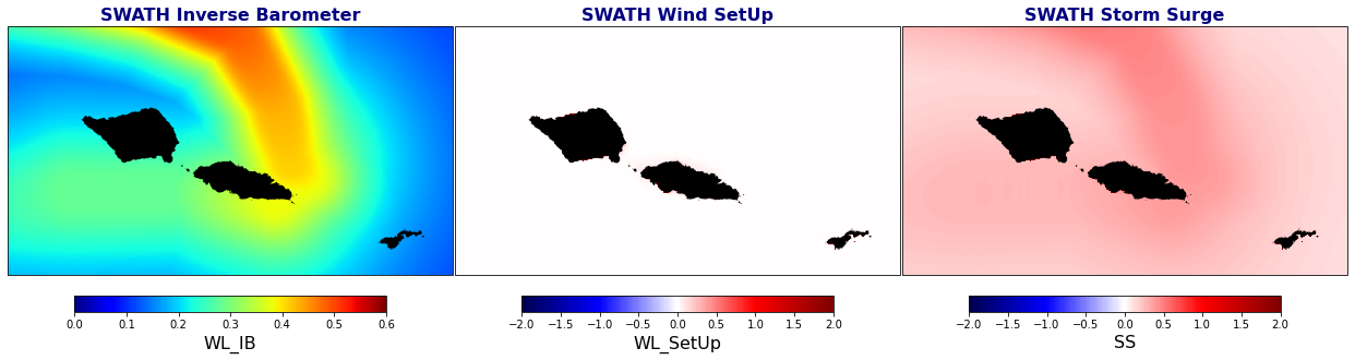
Plot_Grid_TWL_max(TWL, vmax=2, figsize=[22, 12]);
Astronomical Tide#
# domain coordinates
lon_tide_domain = [TWL.lon.min().values-0.5, TWL.lon.max().values+0.5]
lat_tide_domain = [TWL.lat.min().values-0.5, TWL.lat.max().values+0.5]

ds_tide = calculate_AT_TPXO9v4(
    model_directory, lon_tide_domain, lat_tide_domain,
    TWL.time.values[0], TWL.time.values[-1] + np.timedelta64(1, 'h'),
)

ds_tide['lon'] = ds_tide['lon'] + 360

tide = (
    (ds_tide.interpolate_na(dim=('lon'), method='nearest').tide.values) + \
    (ds_tide.interpolate_na(dim=('lat'), method='nearest').tide.values)
)/2

ds_tide['tide'] = (('lat','lon','time'), tide)
TWL['AT'] = (('time','lon', 'lat'), ds_tide.interp(
    lon = TWL.lon.values,
    lat = TWL.lat.values,
    method = 'linear',
).tide.transpose('time','lon','lat').values)
TWL['TWL'] = 0.3 * TWL['Hs'] + TWL['SS'] + TWL['AT']
TWL['TWL_Swath'] = (('lon', 'lat'), TWL.TWL.max(dim='time'))
TWL = TWL.sel(lon=slice(sp_p.lon.min(), sp_p.lon.max()), lat=slice(sp_p.lat.min(), sp_p.lat.max()))
TWL#
TWL
For calculating the total water level (TWL) proxy, we use the following formula:
where the astronomical tide (\(\eta _{AT}\)) is extracted from TOPEX, the storm surge (\(\eta _{SS}\)) from GreenSurge model and \(0.3* H_s\) is a proxy of the setup produced by waves, which are obtained from a combination of SHyTCWaves at a regional scale and downscaled using BinWaves
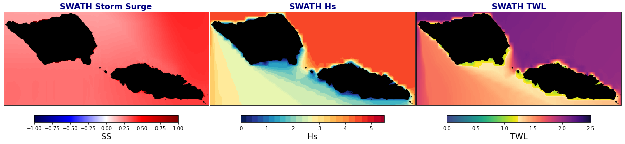
Below are the SWATH maps associated to the Storm Surge (Wind SetUp + Inverse Barometer), Hs, and TWL
Plot_Grid_SWATH(TWL);
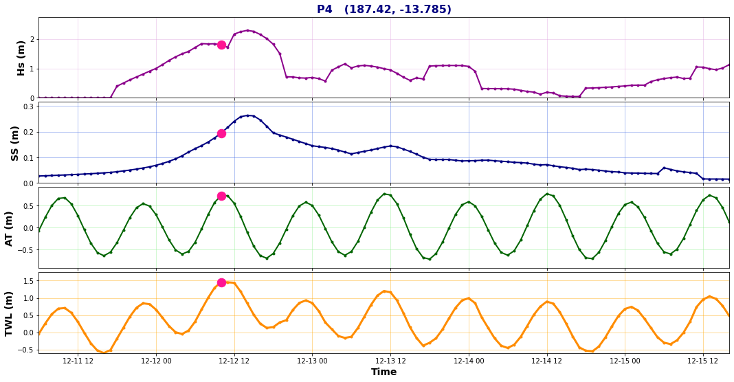
Point Analysis
Below, any point from the ones defined above can be selected to see the evolution of the waves and different level parameters over time.
# point selection
p = 3
p_int = points_interest[0][p] + 360, points_interest[1][p]

twl = TWL.isel(
    lon = np.argmin(np.abs(TWL.lon.values-p_int[0])),
    lat = np.argmin(np.abs(TWL.lat.values-p_int[1])),
)

mp = np.argmax(twl.TWL.values)

print('Point selected: {0}'.format(points_names[p]))
print('Coordinates: {0}'.format(p_int))
Point selected: P4
Coordinates: (187.42, -13.785)
point_code = points_names[p] + '   ' + str(p_int)

Plot_TWL_timeseries(twl, mp, point_code);
Tip
Below there is an animation showing the storm surge (\(\eta _{SS}\)), the astronomical tide (\(\eta _{AT}\)), the \(H_s\) and the combination of the different variables in the TWL.