GreenSurge Validation

# common
import os
import os.path as op
import sys

# pip
import numpy as np
import xarray as xr

# DEV: bluemath
sys.path.insert(0, op.join(op.abspath(''), '..', '..', '..', '..'))

# bluemath modules 
from bluemath.greensurgerepo.storms import historic_track_preprocessing, historic_track_interpolation, get_category
from bluemath.greensurgerepo.vortex import vortex_model_general
from bluemath.greensurgerepo.greensurge import GS_wind_partition, print_GFD_properties, GS_windsetup_reconstruction, presure_to_IB

from bluemath.greensurgerepo.plots.plots_greensurge import plot_case_input, plot_case_vortex_inputs_WP, \
plot_GSdomain_discretization, plot_GS_input_wind_partition, plot_GS_vs_dynamic_windsetup, \
plot_GS_num_validation_timeseries, plot_presure_vs_IB, plot_GS_StormSurge_grafiti, \
plot_GS_TG_validation_timeseries

# hide warnings
import warnings
warnings.filterwarnings('ignore')

## Methodology

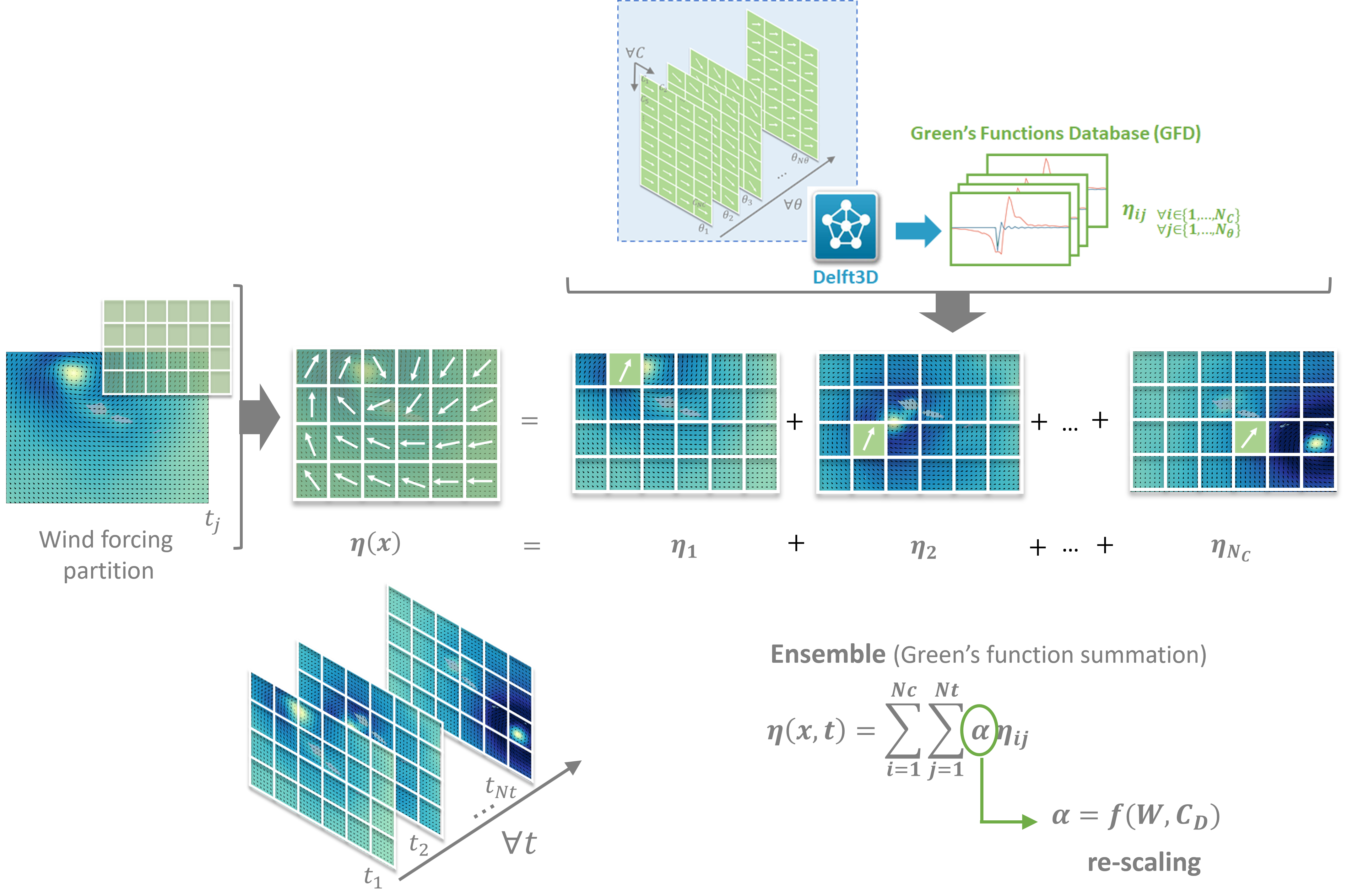
GreenSurge

The Hybrid Modeling of TC-induced Storm Surge surrogate model based on Green’s summation (GreenSurge) and inverse barometer methodology aims to produce accurate estimates of the wind setup and pressure-induced sea level changes due to tropical cyclones (TC) at regional-to-local scales.

Methodology

The steps followed by the GreenSurge methodology, which are exemplified in the figure below, can be summarized as folows:

1. Compilation of the Green’s functions database for the study area.
   

2. Scaling and ensembled from the database to reconstruct any given TC and obtain the induced Wind Setup.
   

3. Obtain the sea level changes due to pressure difference using inverse barometer .
   

4. Obtain the storm surge as the sumation of Wind Set Up and Inverse Barometer .
   

Database and site parameters

# database
p_data = r'/media/administrador/HD2/SamoaTonga/data'
site = 'Samoa'
p_site = op.join(p_data, site)

p_db = r'/media/administrador/HD1/DATABASES'

# deliverable folder
p_deliv = op.join(p_site, 'd06_tc_inundation_forecast')

# ibtracs
p_ibtracs = op.join(p_deliv, 'IBTrACS.ALL.v04r00.nc')

# greensurge library
p_greensurge = op.join(p_db, 'greensurge')
p_GFD_libdir = op.join(p_greensurge, 'GFD_lib', site, 'GFD_Samoa_T84_W40_D15_24h_CDdefault')
domain_study = 'Samoa'

# dynamic simulations
p_TC_Dynamic_Simulations = op.join(p_greensurge, 'data', 'TC_Dynamic_Simulations')

# tidal gauge
p_TC_TG = op.join(p_greensurge, 'data', 'Tidal_Gauge')

Historic TC Analysis

TC data

ibtracs = xr.open_dataset(p_ibtracs)

name = b'EVAN'
TCname = 'EVAN2012'
year = 2020
centerID = 'WMO'

#storm = ibtracs.isel(
#    storm = np.where(
#        (ibtracs.name == name) &  # TODO: necesita \ ?
#        (ibtracs.time[:,0].dt.year.values == year)
#    )[0]
#).isel(storm=0)

storm = ibtracs.isel(storm = 12612)

storm

<xarray.Dataset>
Dimensions:           (date_time: 360, quadrant: 4)
Coordinates:
    time              (date_time) datetime64[ns] 2012-12-10T18:00:00.00003993...
    lat               (date_time) float32 -14.3 -14.55 -14.62 ... nan nan nan
    lon               (date_time) float32 180.2 180.7 181.2 ... nan nan nan
Dimensions without coordinates: date_time, quadrant
Data variables: (12/147)
    numobs            float64 131.0
    sid               |S13 b'2012346S14180'
    season            float64 2.013e+03
    number            int16 88
    basin             (date_time) |S2 b'SP' b'SP' b'SP' b'SP' ... b'' b'' b''
    subbasin          (date_time) |S2 b'MM' b'MM' b'MM' b'MM' ... b'' b'' b''
    ...                ...
    reunion_gust      (date_time) float32 nan nan nan nan ... nan nan nan nan
    reunion_gust_per  (date_time) float32 nan nan nan nan ... nan nan nan nan
    usa_seahgt        (date_time) float32 nan nan nan nan ... nan nan nan nan
    usa_searad        (date_time, quadrant) float32 nan nan nan ... nan nan nan
    storm_speed       (date_time) float32 11.0 11.0 10.0 9.0 ... nan nan nan nan
    storm_dir         (date_time) float32 117.0 108.0 101.0 ... nan nan nan
Attributes: (12/50)
    title:                      IBTrACS - International Best Track Archive fo...
    summary:                    The intent of the IBTrACS project is to overc...
    source:                     The original data are tropical cyclone positi...
    Conventions:                ACDD-1.3
    Conventions_note:           Data are nearly CF-1.7 compliant. The sole is...
    product_version:            v04r00
    ...                         ...
    license:                    These data may be redistributed and used with...
    featureType:                trajectory
    cdm_data_type:              Trajectory
    comment:                    The tracks of TCs generally look like a traje...
    nco_openmp_thread_number:   1
    NCO:                        4.4.3

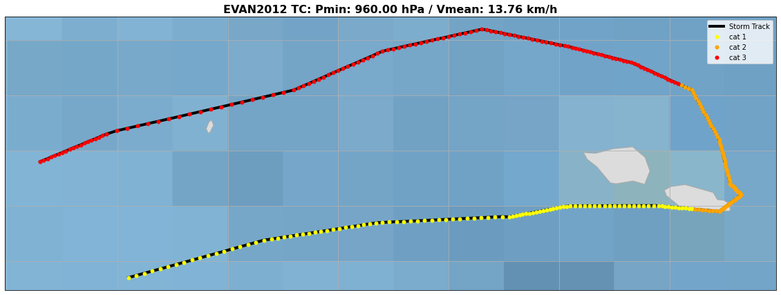
# preprocess selected historic TC: obtain strom variables
df_TC_hist = historic_track_preprocessing(storm, center = centerID)

# computational time step mandatory [60 min] for GS methodology: 
dt_comp = 20 # minutes

# generate interpolated storm track and mandatory data to apply vortex model 
storm_track, time_input = historic_track_interpolation(df_TC_hist, dt_comp)

plot_case_input(storm_track, TCname);

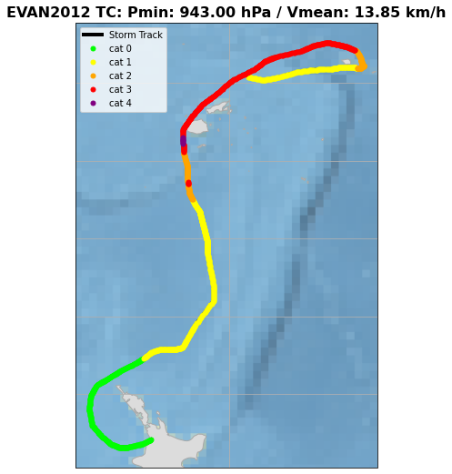
# preprocess selected historic TC: obtain strom variables 
# Storm fraction selection based on temporal coverture (period when the cyclone passes close to Tonga)

# EVAN2012
tini = np.datetime64('2012-12-11T12:00')
tend = np.datetime64('2012-12-15T18:00')

storm_track_sel = storm_track[(storm_track.index >= tini) & (storm_track.index <= tend)]

plot_case_input(storm_track_sel, TCname);

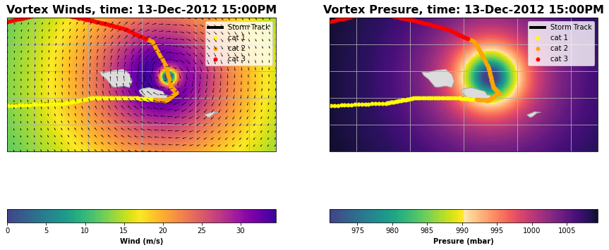
Vortex Model

GreenSurge input: wind fields and sea level preasure from vortex model

# GRID domain study 
Alon = 0.02  # 2km
Alat = 0.02  # 2km

lon = np.linspace(185.5, 190.5, int((190.5-185.5)/Alon)+1)
lat = np.linspace(-15, -12.5, int(abs(-12.5+15)/Alat)+1)

ds_grid_aux = xr.Dataset({
    'lon_grid':(lon),
    'lat_grid':(lat),
})

xds_vortex = vortex_model_general(storm_track_sel, ds_grid_aux)

# Instant
t_num1 = 51

t_num = t_num1 * int(60/dt_comp)

plot_case_vortex_inputs_WP(
    xds_vortex.isel(time = t_num),
    storm_track_sel,
    TCname, 
    mesh = None, 
    quiver = True,
    show_nested = False,
);

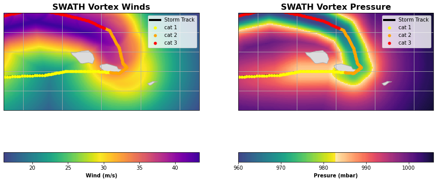
plot_case_vortex_inputs_WP(
    xds_vortex, 
    storm_track_sel,
    TCname,
    swath = True,
    quiver = None,
);

Wind setup

Green Function Dadatabase (GFD)

The first stage, the compilation of the empirical Green’s Functions Database (GFD) includes:

• Definition of the cells for the application of the unit wind covering all possible directions established. The shape and area of these cells should be as small as possible in order to ensure the spatial characterization of any cyclone and large enough not to lose the advantage of this methodology in terms of computing performance and independence with respect to full dynamic simulations.
  

• Definition of the unit wind magnitude and the direction discretization of wind sources, as well as the drag coefficient function (function of wind magnitude).
  

• Time definition of each independent simulation corresponding to each Green’s function, both the length of the sustained unit wind (hereafter, time step) and the time afterwards at which it is necessary to record sea level response over the whole domain.
  

• Computation of the GFD with a SW numerical model.
  

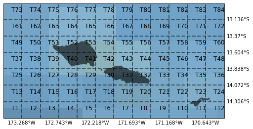
p_GFD_info = op.join(p_GFD_libdir, 'GFD_lib_info.nc')

ds_GFD_info = xr.open_dataset(p_GFD_info) 

print_GFD_properties(ds_GFD_info, domain_study)

plot_GSdomain_discretization(ds_GFD_info);

GFD info: 
--------- 
Samoa domain 
84 cells, 29*25 km resolution 
24 wind directions, 15º resolution 
Unit wind speed: 40m/s 
CD formulation: Wu1982 

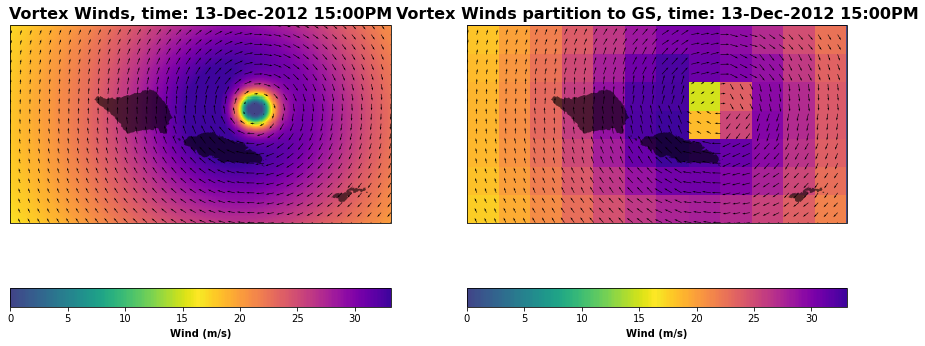
Vortex Wind Fields

The second stage for any TC event study includes:

• Partition of original TC-induced wind fields (regardless of their origin: from parameterizations using Holland vortex model or from forecasting systems) taking into account spatial (i.e. cells) and temporal (i.e. length of sustained winds) resolutions defined in stage 1.
  

• Search for analogues of the above wind forcing partition for each cell and time step in the corresponding forcings of the GFD pre-computed in stage 1. At this point, it is worth mentioning that, since a unit wind is used, the search for analogues is based on wind directions only.
  

• Re-scaling of the corresponding wind setup according to the realistic wind magnitude taking into account the quadratic expression of the wind shear stress used at the free surface boundary condition for the momentum equations.
  

• Summation of the re-scaled wind setup corresponding to the Green’s Fuctions selected by directional analogy for each time step
  

xds_vortex_GS = vortex_model_general(storm_track_sel, ds_GFD_info)

ds_wind_partition = GS_wind_partition(ds_GFD_info, xds_vortex_GS)

plot_GS_input_wind_partition(
    xds_vortex_GS, ds_wind_partition, 
    storm_track_sel, 
    t_num = t_num1 * int(60/dt_comp),
    quiver = True,
);

Run: Searching for analogues, re-scaling and applying wind-drag coefficient

ds_WL_GS_WindSetUp = GS_windsetup_reconstruction(
    p_GFD_libdir, 
    ds_GFD_info,
    ds_wind_partition, 
    xds_vortex_GS,
)

Results: Wind Setup Numeric Validation (Dynamic vs GS)

# Load wind setup dynamic results to compare with GS results
nc_fileID = op.join(p_TC_Dynamic_Simulations, 'ds_{0}_DynamicWindSetUp.nc'.format(TCname))

ds_WL_dynamic_WindSetUp = xr.open_dataset(nc_fileID)

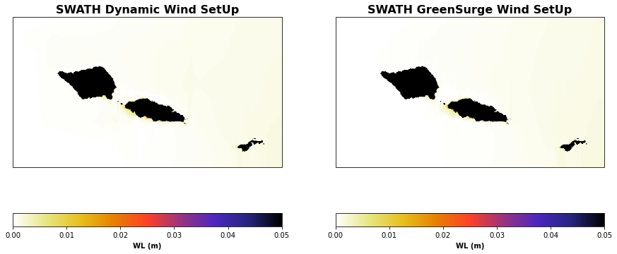
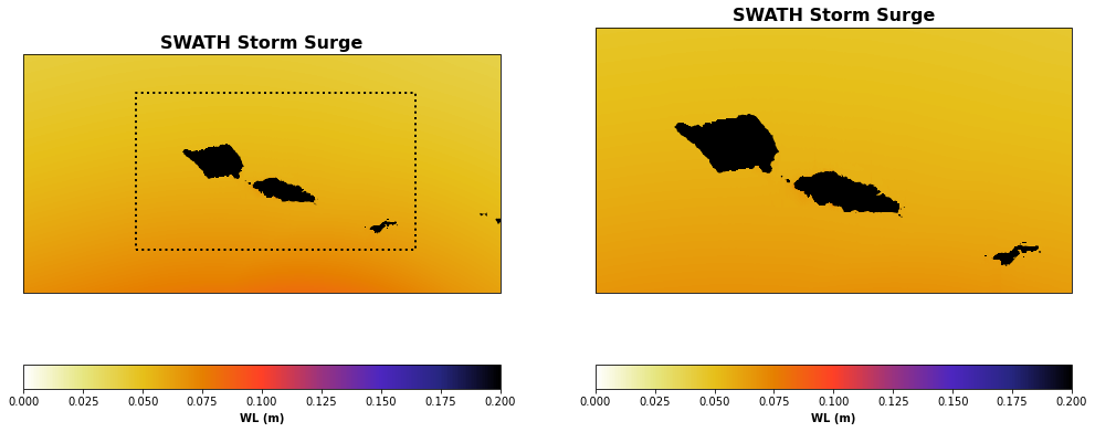
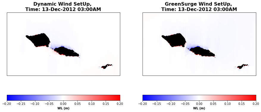
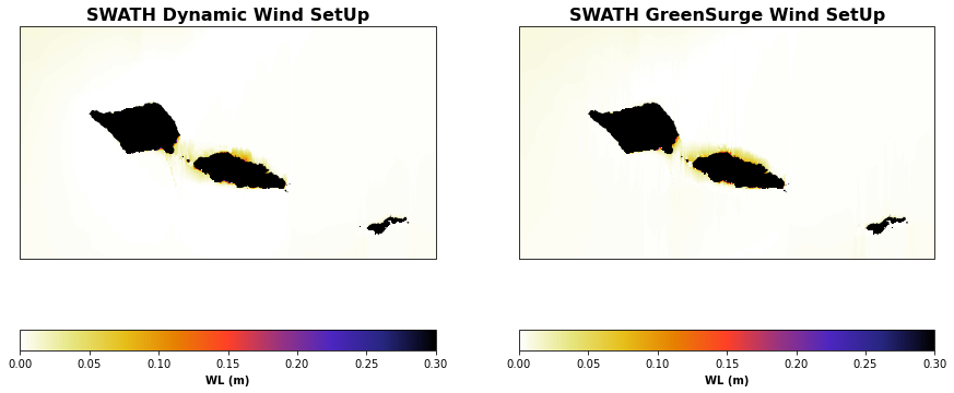
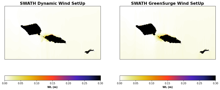
Model validation

The figures below show the maps of a given time and the swath maps of wind setup resulting from dynamic simulations with the Shallow Water Equation (SWE) model Delft3D (left panels) and from the GreenSurge aproach (right panels). These figures illustrate the importance of the wind setup in shallow water areas close to shore (it reaches values up to 0.2m whithin this case) and de acuracy of the GreenSurge approach compared to dynamic simulations.

plot_GS_vs_dynamic_windsetup(
    ds_WL_GS_WindSetUp, ds_WL_dynamic_WindSetUp, 
    storm_track, 
    t_num = t_num1,
    vmin = -0.2,
    vmax = 0.2,
);

plot_GS_vs_dynamic_windsetup(
    ds_WL_GS_WindSetUp, ds_WL_dynamic_WindSetUp, 
    storm_track, 
    swath = True,
    vmin = 0,
    vmax = 0.3,
);

# Points timeseries for comparison
lon_obs_points = [-171.75583333, -172, -172.2]
lat_obs_points = [-13.81916667, -13.819, -13.7]

ds_WL_GS_WindSetUp

<xarray.Dataset>
Dimensions:  (lat: 365, lon: 654, time: 102)
Coordinates:
  * time     (time) datetime64[ns] 2012-12-11T12:00:00 ... 2012-12-15T17:00:00
  * lon      (lon) float64 186.7 186.7 186.7 186.7 ... 189.6 189.6 189.6 189.6
  * lat      (lat) float64 -14.54 -14.54 -14.53 -14.53 ... -12.91 -12.91 -12.9
Data variables:
    WL       (time, lon, lat) float64 0.0 0.0 0.0 ... 7.437e-05 7.797e-05
    land     (lon, lat) float64 nan 1.0 1.0 1.0 1.0 1.0 ... nan nan nan nan nan
    dep      (lon, lat) float32 0.0 5.962e+03 5.945e+03 ... 4.854e+03 4.851e+03

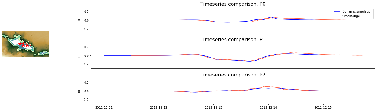
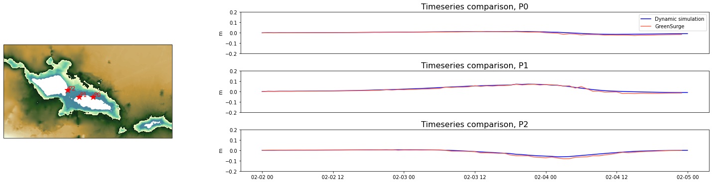
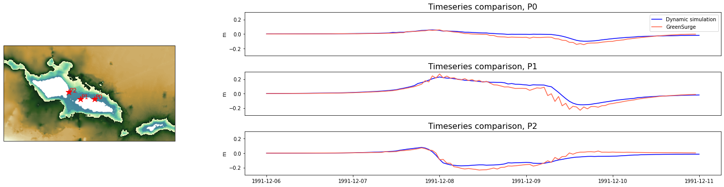
Model validation

The panel below shows timeseries comparison of windsetup at three given locations. These figures illustrate the acuracy of Greensurge approach compared to dynamic simulations.

plot_GS_num_validation_timeseries(
    ds_WL_GS_WindSetUp, ds_WL_dynamic_WindSetUp, 
    lon_obs_points, lat_obs_points,
    figsize = [20,7],
    WLmin = -0.3,
    WLmax = 0.3,
);

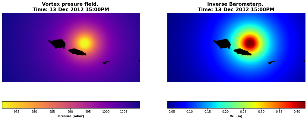
Inverse Barometer

Inverse Barometer

The third stage for any TC event study consist of turning pressure differences into sea level rises and falls using IB methodology which take into account the correlation 1mb-1cm.

Input: Vortex presure fields

# GRID domain study

# HIGHER DEFINITION (spatial and temporal)
Alon = 0.008  # 200m
Alat = 0.008  # 200m

Nlat = int(abs(-12.5+15)/Alat)

lon = np.linspace(185.5, 190.5, int((190.5-185.5)/Alon)+1)
lat = np.linspace(-15, -12.5, int(abs(-12.5+15)/Alat)+1)

ds_grid_aux=xr.Dataset({
    'lon_grid':(lon),
    'lat_grid':(lat),
})

dt_comp = 20 # minutes
storm_track, time_input = historic_track_interpolation(df_TC_hist, dt_comp)
storm_track_sel = storm_track[(storm_track.index >= tini) & (storm_track.index <= tend)]

xds_vortex = vortex_model_general(storm_track_sel, ds_grid_aux)

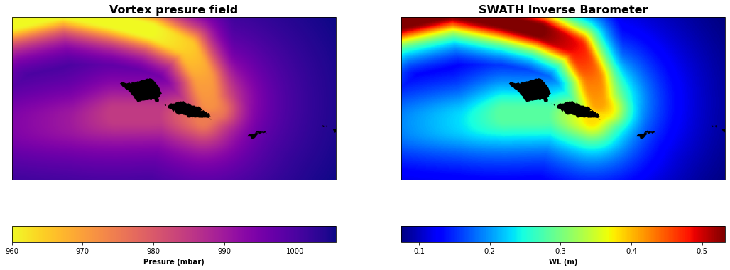
Run and Results

ds_WL_GS_IB = presure_to_IB(xds_vortex)

plot_presure_vs_IB(
    xds_vortex, ds_WL_GS_IB, 
    storm_track, 
    t_num = t_num1*int(60/dt_comp),
);

plot_presure_vs_IB(
    xds_vortex, ds_WL_GS_IB, 
    storm_track, 
    swath = True,
);

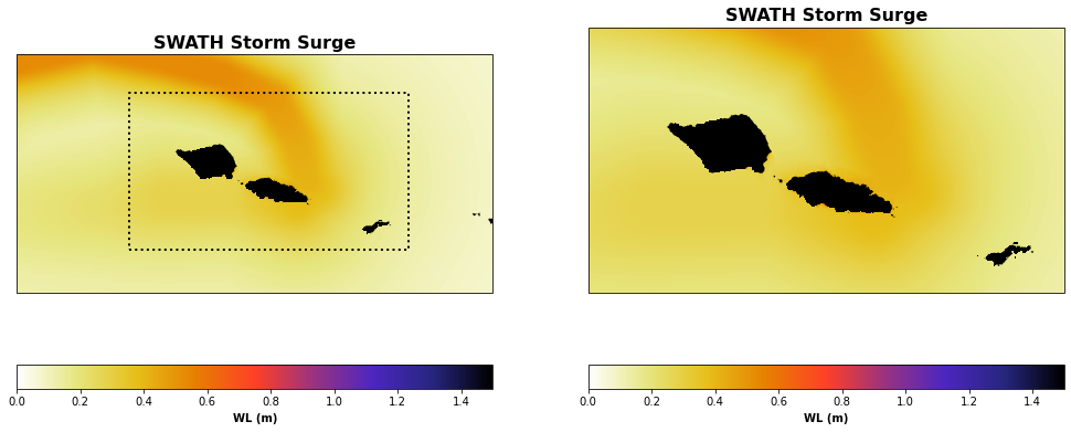
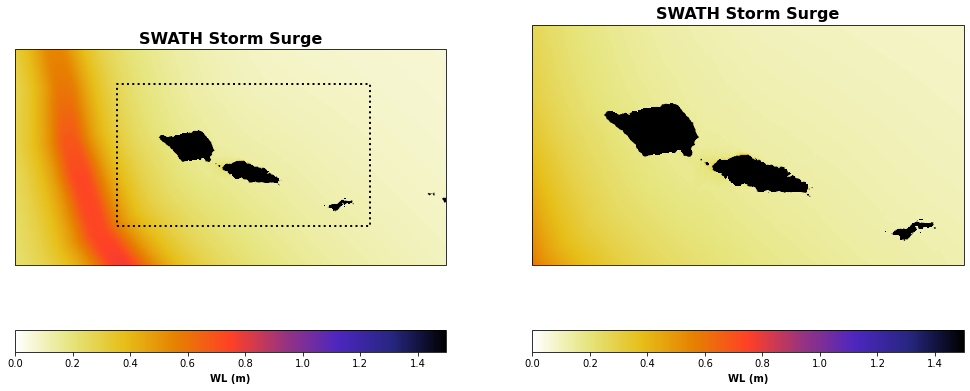
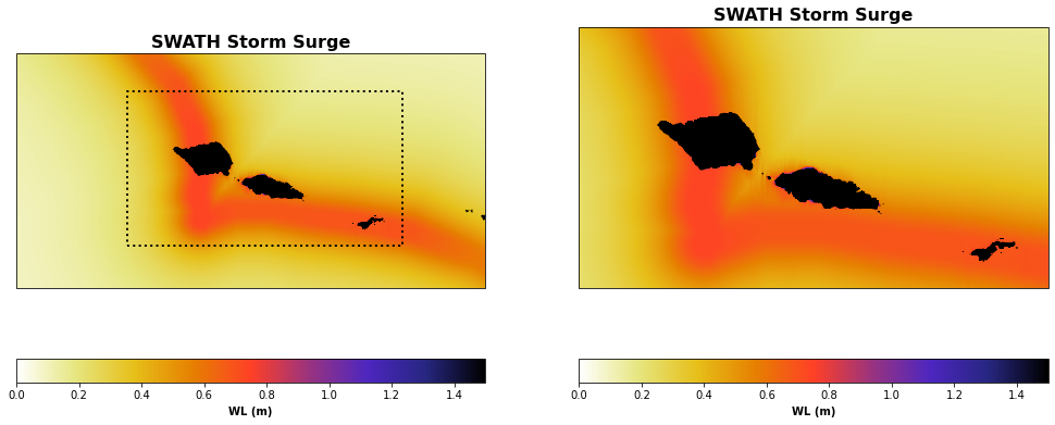
Storm Surge

Storm Surge

Finally the fourth stage sums both components, the wind setup and the pressure-induced sea level changes, to obtain the storm surge.

\[ \eta _{SS} = \eta _{WindSetUp} + \eta _{IB} \]

# Unify meshes to sum components

# base mesh
Alon = 0.002  # 200m
Alat = 0.002  # 200m

lon = np.linspace(185.5, 190.5, int((190.5-185.5)/Alon)+1)
lat = np.linspace(-15, -12.5, int(abs(-12.5+15)/Alat)+1)

ds_grid_GS = xr.Dataset({
    'lon_grid':(lon),
    'lat_grid':(lat),
})

# IB --> base mesh
ds_GS_IB_max = ds_WL_GS_IB.max(dim = 'time')

ds_grid_GS_IB_max = ds_GS_IB_max.interp(
    lat = ds_grid_GS.lat_grid, 
    lon = ds_grid_GS.lon_grid, 
    method = "linear",
)

# Windsetup --> base mesh and higher temporal resolution
ds_GS_WindSetUp_max = ds_WL_GS_WindSetUp.max(dim = 'time')

ds_grid_GS_WindSetUp_max = ds_GS_WindSetUp_max.interp(
    lat = ds_grid_GS.lat_grid,
    lon = ds_grid_GS.lon_grid,
    method = "linear",
    kwargs = {"fill_value":0},
)

#ds_grid_GS_WindSetUp_max = ds_grid_GS_WindSetUp.interp(time=ds_grid_GS_IB.time)

# Components summation
ds_WL_GS_StormSurge_max = ds_grid_GS_IB_max.WL + ds_grid_GS_WindSetUp_max.WL

lon_lims = [min(ds_WL_GS_WindSetUp.lon.values), max(ds_WL_GS_WindSetUp.lon.values)]
lat_lims = [min(ds_WL_GS_WindSetUp.lat.values), max(ds_WL_GS_WindSetUp.lat.values)]

plot_GS_StormSurge_grafiti(
    ds_WL_GS_StormSurge_max, ds_WL_GS_WindSetUp,
    storm_track,
    lon_lims, lat_lims,
    vmin = 0,
    vmax = 1.5,
);

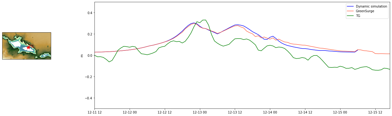
Validation against Tidal Gauge

# Load TG data
p_tg = op.join(p_TC_TG, 'TG_{0}_Samoa.nc'.format(TCname)) 
TG = xr.open_dataset(p_tg)

Model validation

The panel below shows the GreenSurge validation using Tidal Gauge data. This timeseries comparison reveals the good approximation achieved using the GreenSurge approach.

plot_GS_TG_validation_timeseries(
    ds_WL_GS_WindSetUp, ds_WL_GS_IB, 
    ds_WL_dynamic_WindSetUp,
    TG, 
    figsize = [20,7],
    WLmin = -0.5,
    WLmax = 0.5,
);

Validation for Extra TCs

Examples

Here is the validation for some extra TC examples:
-Ofa 1990
-Val 1991
-Winston 2016

Ofa TC (1990)

Val TC (1991)

Winston TC (2016)