SHyTCWaves validation
Contents
SHyTCWaves validation#
# common
import os
import os.path as op
import sys

# pip
import numpy as np
import pandas as pd
import xarray as xr

# DEV: bluemath
sys.path.insert(0, op.join(op.abspath(''), '..', '..', '..', '..'))

# bluemath modules
from bluemath.shytcwaves.storms import check_storm_data, historic_track_preprocessing
from bluemath.shytcwaves.storms import historic_track_interpolation, track_triming

from bluemath.shytcwaves.stopmotion import storm2stopmotion, stopmotion_interpolation, stopmotion_st_bmu, stopmotion_st_spectra
from bluemath.shytcwaves.stopmotion import find_analogue, analogue_endpoints, superpoint_superposition

from bluemath.shytcwaves.plotting.stopmotion import plot_params_analogue, plot_params_anom_series
from bluemath.shytcwaves.plotting.stopmotion import plot_grid_segments, plot_ensemble_val_series, plot_ensemble_val_sp
from bluemath.shytcwaves.plotting.aux_notebook import Plot_st_vars

# hide warnings
import warnings
warnings.filterwarnings('ignore')
Methodology#
SHyTCWaves
The Stop-motion Hybrid TC-induced Waves (SHyTCWaves) surrogate model aims to produce accurate estimates of the directional wave spectra due to a tropical cyclone at the regional scale, which will then serve as the boundary condition for downscaling local waves by means of BinWaves
Methodology
The steps followed by the ShyTCWaves methodology, which are exemplified in the figure below, can be summarized as folows:
Generate library of numerically simulated 6h segments defined by 10 different parameters.
For a given TC, obtain its segments and find the analogue within the library.
Post process and ensemble the different segments to obtain the wave fields at a regional scale and the SuperPoint, as the input for forther downscaling waves.

Database and site parameters#
# database
p_data = r'/media/administrador/HD2/SamoaTonga/data'
site = 'Samoa'
p_site = op.join(p_data, site)

# deliverable folder
p_deliv = op.join(p_site, 'd06_tc_inundation_forecast')
p_db = r'/media/administrador/HD1/DATABASES'

# ibtracs
p_ibtracs = op.join(p_deliv, 'IBTrACS.ALL.v04r00.nc')#'ibtracs.nc')

# evan SWAN case bathymetry
p_proj = op.join(p_deliv, 'projects', 'nb_dyn_evan')
p_bathy = op.join(p_proj, 'depth_evan.nc')
p_swan_output = op.join(p_proj, 'output_main.nc')
p_vortex = op.join(p_proj, 'cases', '0000', 'vortex_wind_main.nc')

# TODO: superpoint?
p_sp_dyn = op.join(p_proj, 'superpoint_samoa.nc')

# stopmotion
p_stopmotion = op.join(p_deliv, 'stopmotion')
p_df_mda = op.join(p_stopmotion, 'shytcwaves_mda.pkl')
p_xds_mda = op.join(p_stopmotion, 'shytcwaves_mda_indices.nc')

p_sm_lib = op.join(p_db, 'ShyTCWaves', 'output')
# p_sm_lib = op.join(p_stopmotion, 'shytcwaves_output')

for f in [p_deliv, p_proj]:
    if not op.isdir(f):
        os.makedirs(f)
Historic TC#
Available agencies track data
xds_ibtracs = xr.open_dataset(p_ibtracs)

name, year = 'EVAN', 2013
storm = xds_ibtracs.sel(
    storm = np.where(
        (xds_ibtracs.name.values == np.bytes_(name)) & \
        (xds_ibtracs.season.values == year)
    )[0]
)

check_storm_data(storm);

Dynamic simulation results#
# load bathymetry
xds_bathy = xr.open_dataset(p_bathy)

lon = xds_bathy.lon.values[:]
lat = xds_bathy.lat.values[:]

# load outputs
xds_dyn = xr.open_dataset(p_swan_output)
xds_vtx = xr.open_dataset(p_vortex)

xds_vtx = xds_vtx.interp(time = xds_dyn.time.values)

# preprocess historic track
df = historic_track_preprocessing(storm, center='WMO')

# interpolate historic track
st, time_input = historic_track_interpolation(df, 20, interpolation=False, mode='mean')

# discard storm coordinates outside domain limits
st_trim = track_triming(st, lat[0], lon[0], lat[-1], lon[-1])
# Plot storm track variables
Plot_st_vars(xds_bathy, xds_vtx, xds_dyn, st_trim);

SHyTCWaves model results#
# load shytcwaves library (mda5000)
df_mda = pd.read_pickle(p_df_mda)
xds_mda = xr.open_dataset(p_xds_mda)  # (shytcwaves: 3 grids)
Stopmotion segmentation
A historic storm is selected from IBTrACS database, and the available data from center X is extracted.
In case there are gaps of data, track coordinates are interpolated at 6h-interval, so that the storm is split into constant segments of 6h according to the SHyTCWaves methodology.
The storm is trimmed by the domain in which it is desired to obtain results (i.e. dynamic simulation boundary limits).
Every 6h target segment is parameterized in terms of 10 parameters: (P,dP,V,dV,W,dW,R,dR,lat,dAng), to obtain the corresponding stopmotion cases.
Finally a list of independent stop-motion events is generated from consecutive parameterized segments. Each stop-motion event has a duration of 3 days: (24h+6h+42h).
# extract historic data from center X
df = historic_track_preprocessing(storm, center='WMO')

# interpolate track coordinates (constant segments)
dt_int_seg = 6 * 60  # 6h interval [minutes]
st, time_input = historic_track_interpolation(
    df, dt_int_seg,
    interpolation = False,
    mode = 'mean',
)

# storm trim within domain (optional)
st_trim = track_triming(st, lat[0], lon[0], lat[-1], lon[-1])

# stopmotion parameterized segments (24h warmup + 6htarget)
df_seg = storm2stopmotion(st_trim)

# generate stopmotion events
st_list, we_list = stopmotion_interpolation(df_seg, st=st_trim)

print('Number of stop-motion segments: {0}'.format(len(st_list)))
Number of stop-motion segments: 31
Analogue segments from library
Once the historical storm has been converted to a set of consecutive parameterized segments, the SHyTCWaves library is accessed to extract the analogue or nearest stop-motion events.
The analogues are obtained with optimization of the euclidean distance in a 10-parametric space.
However, it is possible to apply weighted factors to some parameters, or other alternatives as well.
The geographical endpoints of the original storm track segments are add for georeferencing.
Finally a list is generated of independent stop-motion events corresponding to the analogue parameters and for a duration of 24h+6h+48h.
# analogue indices
ix_weights = [1] * 10
ix = find_analogue(df_mda, df_seg, ix_weights)

# select analogues from dataframe
df_analogue = df_mda.iloc[ix]

# add absolute storm coordinates (from parameterized historic storm)
df_analogue = analogue_endpoints(df_seg, df_analogue)

# stopmotion parameterized events (FOR ANALOGUE SEGMENTS)
st_list_analogue, we_list_analogue = stopmotion_interpolation(df_analogue, st=st_trim)
Plot analogue parameters
plot_params_analogue(
    df_mda, df_seg, df_analogue,
    s = 5,
    ttl1 = 'MDA',
    ttl2 = 'segments',
    c_analogue = 'red',
);

Segments comparison
The SHyTCWaves parameters (Pmin, dP, Vmean, dV, Wmax, dW, Rmw, dR, dAng, latitude) are obtained for (a) the historic track segments, and (b) the library analogue segments. Plots illustrate the evolution of parameters and the absolute anomalies.
# plot analogue params anomalies
fig = plot_params_anom_series(df_seg, df_analogue);

Plot analogue segments
num = 0

xsize_1 = xds_mda.x_size_left.values[num]*10**3
xsize_2 = xds_mda.x_size_right.values[num]*10**3
ysize_1 = xds_mda.y_size_left.values[num]*10**3
ysize_2 = xds_mda.y_size_right.values[num]*10**3
plot_grid_segments(
    st_list_analogue[:30], df_analogue,
    xsize_1, xsize_2, ysize_1, ysize_2,
    st = st_trim[:30],
    st_list_0 = st_list[:30],
    df_seg_0 = df_seg,
    n_rows = 3, n_cols = 10,
    width = 20, height = 6,
);


Ensemble of analogue segments
This code allows for obtaining results very fast, with minimum computational effort.
For that purpose, a mask is employed to directly locate the relative position of the target control point to the center of the target segment (analogue case). It is convenient to remember that library cases output points are distributed in a polar grid system, so it is possible to assign a mask of radii and angles.
Moreover, a separate file was previously generated with the directional spectra reconstructed Hs, for each case of the library (point,time).
From the reconstructed Hs, and by piling the total number of segments for a given storm track, the best match unit (bmu) that defines the energy enevolpe is found.
Finally, the envelope shytcwaves spectra is obtained by applying the location mask, and the bmu over the analogue cases directional spectra.
Extract bulk envelope
swath_resolution = .4    # [º]

# generate meshgrid
mesh_sw_lon = np.arange(lon[0], lon[-1], swath_resolution)
mesh_sw_lat = np.arange(lat[0], lat[-1], swath_resolution)
mesh_lo, mesh_la = np.meshgrid(mesh_sw_lon, mesh_sw_lat)

print('Number of nodes: {0}'.format(mesh_lo.size))

# extract shytcwaves envelope (bulk)
xds_shy_bulk = stopmotion_st_bmu(
    p_sm_lib,
    df_analogue, df_seg,
    p_stopmotion,
    st_trim,
    list(np.ravel(mesh_lo)), list(np.ravel(mesh_la)),
    max_dist = 60,
)
Number of nodes: 2320
100%|███████████████████████████████████████████| 31/31 [01:11<00:00, 2.30s/it]
Merging bulk envelope... 2022-04-06 16:16:00.787083
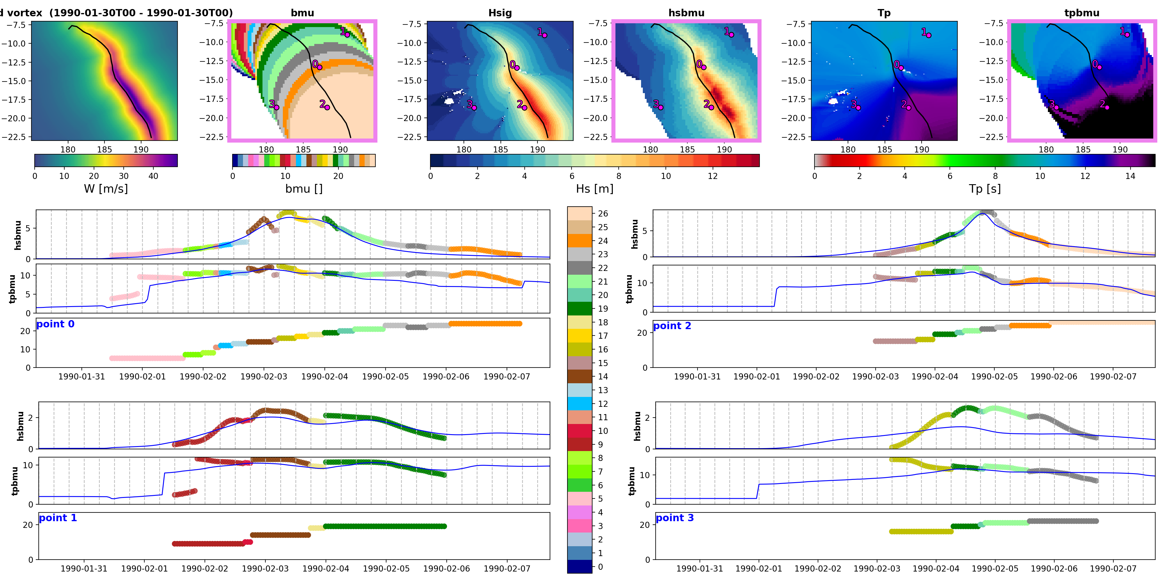
Plot ensemble - validation (SERIES)
Model validation
The panel below shows the swath maps of vortex winds, significant wave height and peak period (comparing dynamic and model results, left and right respectively). The time series panels illustrate the accuracy of the SHyTCWaves model (color dots) compared to dynamic simulations (blue line). Discrepancies may account for island masking.
lonpts = [187.2, 190.9459, 188.2099, 181.3700]
latpts = [-13.35, -9.0125, -18.6247, -18.6247]

plot_ensemble_val_series(
    st_trim,
    xds_shy_bulk, xds_dyn, xds_vtx,
    mesh_lo, mesh_la,
    lonpts, latpts,
    width=20, height=10,
);

SuperPoint
For ShyTCWaves to serve as the input to generate downscaled waves at a local scale, the SuperPoint spectra needs to be obtained at the same locations in which BinWaves model was fitted.
# control points (Samoa superpoint)
lo_2191, la_2191 = 186.87, -12.93
lo_2193, la_2193 = 187.93, -12.93
lo_2195, la_2195 = 189.00, -12.93
lo_2183, la_2183 = 186.87, -13.47
lo_2187, la_2187 = 189.00, -13.47
lo_2175, la_2175 = 186.87, -14
lo_2178, la_2178 = 189.00, -14
lo_2166, la_2166 = 186.87, -14.53
lo_2168, la_2168 = 187.93, -14.53
lo_2170, la_2170 = 189.00, -14.53

lonpts = [lo_2191,lo_2193,lo_2195,lo_2183,lo_2187,lo_2175,lo_2178,lo_2166,lo_2168,lo_2170]
latpts = [la_2191,la_2193,la_2195,la_2183,la_2187,la_2175,la_2178,la_2166,la_2168,la_2170]
namepts = ['2191','2193','2195','2183','2187','2175','2178','2166','2168','2170']

print('Number of nodes: {0}'.format(len(lonpts)))

xds_shy_spec, _ = stopmotion_st_spectra(
    p_sm_lib,
    df_analogue, df_seg,
    p_stopmotion,
    st_trim,
    lonpts, latpts,
    cp_names = namepts,
    max_dist = 60,
    list_out = False,
)
Number of nodes: 10
100%|███████████████████████████████████████████| 31/31 [00:46<00:00, 1.52s/it]
Merging bulk envelope... 2022-04-06 16:16:51.468954
100%|███████████████████████████████████████████| 31/31 [04:07<00:00, 7.99s/it]
Inserting envelope spectra... 2022-04-06 16:20:59.386053
Build Superpoint#
# SAMOA
deg_sup = 9     # Degrees of superposition
stations = list(np.arange(0, xds_shy_spec.point.size))   # 91,93,95,83,87,75,78,66,68,70
sectors = [
    (306, 342),
    (342, 18),
    (18, 54),
    (270, 306),
    (54, 90),
    (234, 270),
    (90, 126),
    (198, 234),
    (162, 198),
    (126, 162),
]  # 10 sectors (36º)

# positions of the stations for plotting
pos_st = [1, 2, 3, 0, 4, 5, 9, 6, 7, 8]   # 17,14,15,16,18,19,21,22,23,20

# superpoint superposition
xds_shy_sp = superpoint_superposition(xds_shy_spec, stations, sectors, deg_sup)
Plot ensemble - validation (SWATH)
Model validation
The panel below shows the swath maps of vortex winds, significant wave height and peak period (comparing dynamic and model results, upper and middle rows respectively). Lower row compares the swath directional wave spectra of the superpoint, and the difference.
xds_dyn_sp = xr.open_dataset(p_sp_dyn)

fig = plot_ensemble_val_sp(
    st_trim,
    xds_shy_bulk, xds_shy_sp,
    xds_vtx, xds_dyn, xds_dyn_sp,
    mesh_lo, mesh_la,
    spec_max = 1,
    swath = True,
    width = 20,
    height = 15,
)

Examples
Here is the validation for some extra TC examples:
Ofa 1990
Winston 2016
OFA 1990:
WINSTON 2016:
