Computational Complexity
Computational complexity is a field from computer science which analyzes algorithms based on the amount resources required for running it. The amount of required resources varies based on the input size, so the complexity is generally expressed as a function of \(n\), where \(n\) is the size of the input.
It is important to note that when analyzing an algorithm we can consider the time complexity and space complexity. The space complexity is basically the amount of memory space required to solve a problem in relation to the input size. Even though the space complexity is important when analyzing an algorithm, in this section we will focus only on the time complexity.
In computer science, the time complexity is the computational complexity that describes the amount of time it takes to run an algorithm. Time complexity is commonly estimated by counting the number of elementary operations performed by the algorithm, supposing that each elementary operation takes a fixed amount of time to perform.
When analyzing the time complexity of an algorithm we may find three cases: best-case, average-case and worst-case. Let’s understand what it means.
Suppose we have the following unsorted list [1, 5, 3, 9, 2, 4, 6, 7, 8] and we need to find the index of a value in this list using linear search.
- best-case: this is the complexity of solving the problem for the best input. In our example, the best case would be to search for the value 1. Since this is the first value of the list, it would be found in the first iteration.
- average-case: this is the average complexity of solving the problem. This complexity is defined with respect to the distribution of the values in the input data. Maybe this is not the best example but, based on our sample, we could say that the average-case would be when we’re searching for some value in the “middle” of the list, for example, the value 2.
- worst-case: this is the complexity of solving the problem for the worst input of size n. In our example, the worst-case would be to search for the value 8, which is the last element from the list.
Usually, when describing the time complexity of an algorithm, we are talking about the worst-case. To describe the time complexity of an algorithm we use a mathematical notation called Big-O.
Mathematically the complexity of a function is the relationship between the size of the input and the difficulty of running the function to completion. The size of the input is usually denoted by \(n\). However, \(n\) usually describes something more tangible, such as the length of an array. The difficulty of a problem can be measured in several ways. One suitable way to describe the difficulty of the problem is to use basic operations: additions, subtractions, multiplications, divisions, assignments, and function calls. Although each basic operation takes different amounts of time, the number of basic operations needed to complete a function is sufficiently related to the running time to be useful, and it is much easier to count.
Example: Count the number of basic operations, in terms of \(n\), required for the following function to terminate.
def f(n):
    out = 0
    for i in range(n):
        for j in range(n):
            out += i*j

    return out
Let’s calculate the number of operations:
additions: \(n^2\), subtractions: 0, multiplications: \(n^2\), divisions: 0, assignments: \(2n^2 +1\), function calls: 0, total: \(4n^2+1\).
The number of assignments is \(2n^2 + n + 1\) because the line \(out += i*j\) is evaluated \(n^2\) times, \(j\) is assigned \(n^2\), \(i\) is assigned \(n\) times, and the line \(out = 0\) is assigned once. So, the complexity of the function \(f\) can be described as \(4n^2 + n + 1\).
A common notation for complexity is called Big-O notation. Big-O notation establishes the relationship in the growth of the number of basic operations with respect to the size of the input as the input size becomes very large. Since hardware is different on every machine, we cannot accurately calculate how long it will take to complete without also evaluating the hardware. Then that analysis is only good for that specific machine. We do not really care how long a specific set of input on a specific machine takes. Instead, we will analyze how quickly “time to completion” in terms of basic operations grows as the input size grows, because this analysis is hardware independent. As \(n\) gets large, the highest power dominates; therefore, only the highest power term is included in Big-O notation. Additionally, coefficients are not required to characterize growth, and so coefficients are also dropped. In the previous example, we counted \(4n^2 + n + 1\) basic operations to complete the function. In Big-O notation we would say that the function is \(O(n^2)\) (pronounced “O of n-squared”). We say that any algorithm with complexity \(O(nc)\) where \(c\) is some constant with respect to \(n\) is polynomial time.
Example: Determine the complexity of the iterative Fibonacci function in Big-O notation.
def my_fib_iter(n):

    out = [1, 1]

    for i in range(2, n):
        out.append(out[i - 1] + out[i - 2])

    return out
Since the only lines of code that take more time as \(n\) grows are those in the for-loop, we can restrict our attention to the for-loop and the code block within it. The code within the for-loop does not grow with respect to \(n\) (i.e., it is constant). Therefore, the number of basic operations is \(Cn\) where \(C\) is some constant representing the number of basic operations that occur in the for-loop, and these \(C\) operations run \(n\) times. This gives a linear time complexity of \(O(n)\) for \(my\_fib\_iter\).
Assessing the exact complexity of a function can be difficult. In these cases, it might be sufficient to give an upper bound or even an approximation of the complexity.
Example: Give an upper bound on the complexity of the recursive implementation of Fibonacci. Do you think it is a good approximation of the upper bound? Do you think that recursive Fibonacci could possibly be polynomial time?
def my_fib_rec(n):

    if n < 2:
        out = 1
    else:
        out = my_fib_rec(n-1) + my_fib_rec(n-2)

    return out
As \(n\) gets large, we can say that the vast majority of function calls make two other function calls: one addition and one assignment to the output. The addition and assignment do not grow with \(n\) per function call, so we can ignore them in Big-O notation. However, the number of function calls grows approximately by \(2^n\) , and so the complexity of \(my\_fib\_rec\) is upper bound by \(O(2^n)\).
There is on-going debate whether or not \(O(2^n)\) is a good approximation for the Fibonacci function.
Since the number of recursive calls grows exponentially with \(n\), there is no way the recursive fibonacci function could be polynomial. That is, for any \(c\), there is an \(n\) such that \(my\_fib\_rec\) takes more than \(O(n^c)\) basic operations to complete. Any function that is \(O(c^n)\) for some constant c is said to be exponential time.
Example: What is the complexity of the following function in Big-O notation?
def my_divide_by_two(n):

    out = 0
    while n > 1:
        n /= 2
        out += 1

    return out
Again, only the while-loop runs longer for larger \(n\) so we can restrict our attention there. Within the while-loop, there are two assignments: one division and one addition, which are both constant time with respect to \(n\). So the complexity depends only on how many times the while-loop runs.
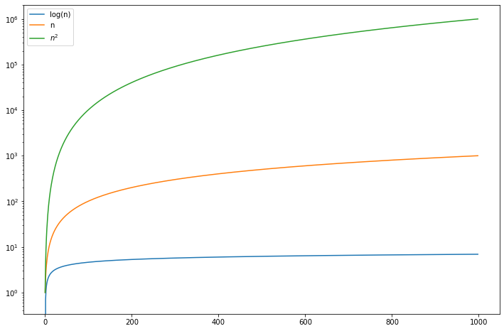
The while-loop cuts \(n\) in half in every iteration until \(n\) is less than 1. So the number of iterations, \(I\), is the solution to the equation \(\frac{n}{2^I} = 1\). With some manipulation, this solves to \(I = \log n\), so the complexity of \(my\_divide\_by\_two\) is \(O(\log n)\). It does not matter what the base of the log is because, recalling log rules, all logs are a scalar multiple of each other. Any function with complexity \(O(\log n)\). is said to be log time.
A graphical comparison of the complexity for different input size is:
import numpy as np
import matplotlib.pyplot as plt

plt.figure(figsize = (12, 8))
n = np.arange(1, 1e3)
plt.plot(np.log(n), label = 'log(n)')
plt.plot(n, label = 'n')
plt.plot(n**2, label = '$n^2$')
#plt.plot(2**n, label = '$2^n$')
plt.yscale('log')
plt.legend()
plt.show()
These are the most common time complexities expressed using the Big-O notation:
╔══════════════════╦═════════════════╗
║       Name       ║ Time Complexity ║
╠══════════════════╬═════════════════╣
║ Constant Time    ║       O(1)      ║
╠══════════════════╬═════════════════╣
║ Logarithmic Time ║     O(log n)    ║
╠══════════════════╬═════════════════╣
║ Linear Time      ║       O(n)      ║
╠══════════════════╬═════════════════╣
║ Quasilinear Time ║    O(n log n)   ║
╠══════════════════╬═════════════════╣
║ Quadratic Time   ║      O(n^2)     ║
╠══════════════════╬═════════════════╣
║ Exponential Time ║      O(2^n)     ║
╠══════════════════╬═════════════════╣
║ Factorial Time   ║       O(n!)     ║
╚══════════════════╩═════════════════╝
Time Complexities
Constant Time — O(1)
An algorithm is said to have a constant time when it is not dependent on the input data (n). Example: the function get_first which returns the first element of a list:
def get_first(data):
    return data[0]

if __name__ == '__main__':
    data = [1, 2, 9, 8, 3, 4, 7, 6, 5]
    print(get_first(data))
Logarithmic Time — O(log n)
An algorithm is said to have a logarithmic time complexity when it reduces the size of the input data in each step (it don’t need to look at all values of the input data) Example: Algorithms with logarithmic time complexity are commonly found in operations on binary trees or when using binary search. Below is the example of a binary search, where we need to find the position of an element in a sorted list:
def binary_search(data, value):
    n = len(data)
    left = 0
    right = n - 1
    while left <= right:
        middle = (left + right) // 2
        if value < data[middle]:
            right = middle - 1
        elif value > data[middle]:
            left = middle + 1
        else:
            return middle
    raise ValueError('Value is not in the list')

if __name__ == '__main__':
    data = [1, 2, 3, 4, 5, 6, 7, 8, 9]
    print(binary_search(data, 8))
Linear Time — O(n)
An algorithm is said to have a linear time complexity when the running time increases at most linearly with the size of the input data. This is the best possible time complexity when the algorithm must examine all values in the input data. Example: a linear search, where we need to find the position of an element in an unsorted list
def linear_search(data, value):
    for index in range(len(data)):
        if value == data[index]:
            return index
    raise ValueError('Value not found in the list')

if __name__ == '__main__':
    data = [1, 2, 9, 8, 3, 4, 7, 6, 5]
    print(linear_search(data, 7))
Quasilinear Time — O(n log n)
An algorithm is said to have a quasilinear time complexity when each operation in the input data have a logarithm time complexity. It is commonly seen in sorting algorithms (e.g. mergesort, heapsort). Example: the Mergesort algorithm is an efficient, general-purpose, comparison-based sorting algorithm which has quasilinear time complexity:
def merge_sort(data):
    if len(data) <= 1:
        return

    mid = len(data) // 2
    left_data = data[:mid]
    right_data = data[mid:]

    merge_sort(left_data)
    merge_sort(right_data)

    left_index = 0
    right_index = 0
    data_index = 0

    while left_index < len(left_data) and right_index < len(right_data):
        if left_data[left_index] < right_data[right_index]:
            data[data_index] = left_data[left_index]
            left_index += 1
        else:
            data[data_index] = right_data[right_index]
            right_index += 1
        data_index += 1

    if left_index < len(left_data):
        del data[data_index:]
        data += left_data[left_index:]
    elif right_index < len(right_data):
        del data[data_index:]
        data += right_data[right_index:]

if __name__ == '__main__':
    data = [9, 1, 7, 6, 2, 8, 5, 3, 4, 0]
    merge_sort(data)
    print(data)
Quadratic Time — O(n²)
An algorithm is said to have a quadratic time complexity when it needs to perform a linear time operation for each value in the input data. Example: Bubble sort is a great example of quadratic time complexity since for each value it needs to compare to all other values in the list:
def bubble_sort(data):
    swapped = True
    while swapped:
        swapped = False
        for i in range(len(data)-1):
            if data[i] > data[i+1]:
                data[i], data[i+1] = data[i+1], data[i]
                swapped = True

if __name__ == '__main__':
    data = [9, 1, 7, 6, 2, 8, 5, 3, 4, 0]
    bubble_sort(data)
    print(data)
Exponential Time — O(2^n)
An algorithm is said to have an exponential time complexity when the growth doubles with each addition to the input data set. Example: recursive calculation of Fibonacci numbers:
def fibonacci(n):
    if n <= 1:
        return n
    return fibonacci(n-1) + fibonacci(n-2)
Factorial — O(n!)
An algorithm is said to have a factorial time complexity when it grows in a factorial way based on the size of the input data. Example: an algorithm which has a factorial time complexity is the Heap’s algorithm, which is used for generating all possible permutations of n objects.
def heap_permutation(data, n):
    if n == 1:
        print(data)
        return

    for i in range(n):
        heap_permutation(data, n - 1)
        if n % 2 == 0:
            data[i], data[n-1] = data[n-1], data[i]
        else:
            data[0], data[n-1] = data[n-1], data[0]

if __name__ == '__main__':
    data = [1, 2, 3]
    heap_permutation(data, len(data))
Another great example is the Travelling Salesman Problem.
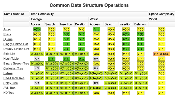
You can find below a sheet with the time complexity of the operations in the most common data structures.
Python Elapsed Time Functions
It often helps to know how long certain sections of code require to run
import time
start = time.time()
# some code to time
end = time.time()
elapsed = end-start
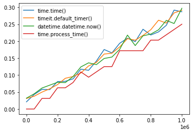
Example: It is shown below how to implement a simple timer on sections of code
import time
import timeit
import datetime

def concat1(n):
    start = time.time()
    time.sleep(0.02)
    s = "-".join(str(i) for i in range(n))
    end = time.time()
    return end-start

def concat2(n):
    start = timeit.default_timer()
    time.sleep(0.02)
    s = "-".join(str(i) for i in range(n))
    end = timeit.default_timer()
    return end-start

def concat3(n):
    start = datetime.datetime.now()
    time.sleep(0.02)
    s = "-".join(str(i) for i in range(n))
    end = datetime.datetime.now()
    return (end-start).total_seconds()

def concat4(n):
    start = time.process_time()
    time.sleep(0.02)
    s = "-".join(str(i) for i in range(n))
    end = time.process_time()
    return end-start

print(timeit.timeit('"-".join(str(i) for i in range(100000))',number=5))
print(concat1(100000))
print(concat2(100000))
print(concat3(100000))
print(concat4(100000))

import numpy as np
x = np.arange(1,1000002,50000)
y1 = np.empty(len(x))
y2 = np.empty(len(x))
y3 = np.empty(len(x))
y4 = np.empty(len(x))
for j,xj in enumerate(x):
    y1[j] = concat1(xj)
    y2[j] = concat2(xj)
    y3[j] = concat3(xj)
    y4[j] = concat4(xj)
    print(j,xj,y1[j],y2[j],y3[j],y4[j])

import matplotlib.pyplot as plt
plt.plot(x,y1,label='time.time()')
plt.plot(x,y2,label='timeit.default_timer()')
plt.plot(x,y3,label='datetime.datetime.now()')
plt.plot(x,y4,label='time.process_time()')
plt.legend()
plt.show()
Comparison of Sorting Algorithms - Time Complexity
Below we can test 9 algorithms (Bubble Sort, Insertion Sort, Selection Sort, Quick Sort, Merge Sort, Heap Sort, Counting Sort, Radix Sort, Bucket Sort ) featured here under a variety of circumstances. From 100 numbers to 10,000 as well as tests using already sorted data, these tests will reveal quite a bit.
The Python timeit and random library were used to generate the random data, and perform continuous and repeated tests for each algorithm. This is again, to ensure fair results. The Random library is used to generate numbers from 1 to 10,000 and the timeit library performs each test 5 times in total, and returns a list of all 5 times. Each one of the 5 tests is actually running the code 10 times, (the number parameter, default value 1,000,000). This increases the accuracy by doing alot of tests and adding together the values to average it out. If you want the individual time for one single sort, divide the min/max value by 10. The number of repetitions is controlled by the repeat parameter (default value 5). Below it is shown the code for all algorithms and the setup for radix sort:
def bubbleSort(arr):
    n = len(arr)

    for i in range(n-1):
        for j in range(0, n-i-1):
            if arr[j] > arr[j+1] :
                arr[j], arr[j+1] = arr[j+1], arr[j]
    return arr

def bubbleSort_unoptimized(arr):
    n = len(arr)

    for i in range(n-1):
        for j in range(0, n-1):
            if arr[j] > arr[j+1] :
                temp = arr[j]
                arr[j]=  arr[j+1]
                arr[j + 1] = temp
    return arr

def bubbleSort_recursive(arr, n):
    if (n <= 1):
        return arr

    for j in range(0, n-1):
        if arr[j] > arr[j+1] :
            temp = arr[j]
            arr[j]=  arr[j+1]
            arr[j + 1] = temp

    bubbleSort_recursive(arr, n - 1)
    return arr

def insertion_sort(array):

    for i in range(1, len(array)):
        sort_value = array[i]

        while array[i-1] > sort_value and i > 0:
            array[i], array[i-1] = array[i-1], array[i]
            i = i - 1
    return array

def selection_sort(arr):
    for i in range (0, len(arr) - 1):
        minIndex = i
        for j in range (i+1, len(arr)):
            if arr[j] < arr[minIndex]:
                minIndex = j
        if minIndex != i:
            arr[i], arr[minIndex] = arr[minIndex], arr[i]

def Qsort(array, low, high):
    if (low < high):
        pivot = low
        i = low
        j = high

        while (i < j):     # Main While Loop
            while array[i] <= array[pivot] and i < high:    # While Loop "i"
                i += 1
            while array[j] > array[pivot]:                  # While Loop "j"
                j -= 1

            if (i < j):
                array[i], array[j] = array[j], array[i]

        array[pivot], array[j] = array[j], array[pivot]
        Qsort(array, low, j - 1)
        Qsort(array, j + 1, high)
        return array

    else:
      return array

def Qsort_alt(array):
  lesser = []
  greater = []
  equal = []

  if len(array) > 1:
    pivot = array[0]
    for x in array:
      if x < pivot:
        lesser.append(x)
      if x > pivot:
        greater.append(x)
      if x == pivot:
        equal.append(x)
    return Qsort_alt(lesser) + equal + Qsort_alt(greater)
  else:
    return array

def mergesort(x):
    if len(x) < 2:               # Return if array was reduced to size 1
        return x

    result = []                  # Array in which sorted values will be inserted
    mid = int(len(x) / 2)

    y = mergesort(x[:mid])       # 1st half of array
    z = mergesort(x[mid:])       # 2nd half of array
    i = 0
    j = 0
    while i < len(y) and j < len(z):  # Stop if either half reaches its end
        if y[i] > z[j]:
            result.append(z[j])
            j += 1
        else:
            result.append(y[i])
            i += 1
    result += y[i:]             # Add left over elements
    result += z[j:]             # Add left over elements
    return result

def max_heapify(arr,n,i):
    l = 2 * i + 1
    r = 2 * i + 2

    if l < n and arr[l] > arr[i]:
        largest = l
    else:
        largest = i

    if r < n and arr[r] > arr[largest]:
        largest = r

    if largest != i:
        arr[i], arr[largest] = arr[largest], arr[i]
        max_heapify(arr, n, largest)


def build_heap(arr):
    n = len(arr)

    for i in range(n, -1,-1):
        max_heapify(arr, n, i)

    for i in range(n-1,0,-1):
        arr[0] ,arr[i] = arr[i], arr[0]
        max_heapify(arr, i, 0)

def counting(data):
    # Creates 2D list of size max number in the array
    counts = [0 for i in range(max(data)+1)]
    print(counts)

    # Finds the "counts" for each individual number
    for value in data:
        counts[value] += 1
    print(counts)

    # Finds the cumulative sum counts
    for index in range(1, len(counts)):
        counts[index] = counts[index-1] + counts[index]
    print(counts)

    # Sorting Phase
    arr = [0 for loop in range(len(data))]
    for value in data:
        index = counts[value] - 1
        arr[index] = value
        counts[value] -= 1

    return arr

# get number of digits in largest item
def num_digits(arr):
    maxDigit = 0
    for num in arr:
        maxDigit = max(maxDigit, num)
    return len(str(maxDigit))


# flatten into a 1D List
from functools import reduce
def flatten(arr):
    return reduce(lambda x, y: x + y, arr)


def radix(arr):
    digits = num_digits(arr)
    for digit in range(0, digits):
        temp = [[] for i in range(10)]
        for item in arr:
            num = (item // (10 ** digit)) % 10
            temp[num].append(item)
        arr = flatten(temp)
    return arr


def bucketSort(array):
    largest = max(array)
    length = len(array)
    size = largest/length

    # Create Buckets
    buckets = [[] for i in range(length)]

    # Bucket Sorting
    for i in range(length):
        index = int(array[i]/size)
        if index != length:
            buckets[index].append(array[i])
        else:
            buckets[length - 1].append(array[i])

    # Sorting Individual Buckets
    for i in range(len(array)):
        buckets[i] = sorted(buckets[i])


    # Flattening the Array
    result = []
    for i in range(length):
        result = result + buckets[i]

    return result

import timeit

def test():
    SETUP_CODE = '''
from __main__ import radix
from random import shuffle'''

    TEST_CODE = '''
n = 1000
array = [x for x in range(n)]
shuffle(array)
radix(array)
  '''
    times = timeit.repeat( setup = SETUP_CODE,stmt = TEST_CODE, number = 10,repeat = 5)
    print('Min Time: {}'.format(min(times)))
    print('Max Time: {}'.format(max(times)))


if __name__ == "__main__":
    # array = [3, 6, 1, 2, 8, 4, 6]
    # print(bubbleSort(array))
    # array = [3, 6, 1, 2, 8, 4, 6]
    # print(bubbleSort_unoptimized(array))
    # array = [3, 6, 1, 2, 8, 4, 6]
    # print(bubbleSort_recursive(array, len(array) - 1))
    # A = [4,6,8,3,2,5,7,9,0]
    # print(insertion_sort(A))
    # nums = [5,9,1,2,4,8,6,3,7]
    # selection_sort(nums)
    # print(nums)
    # A = [4,6,8,3,2,5,7,9,0]
    # print(Qsort(A,0,len(A) - 1))
    # A = [4,6,8,3,2,5,7,9,0]
    # print(mergesort(A))
    # arr = [33,35,42,10,7,8,14,19,48]
    # build_heap(arr)
    # print(arr)
    # data = [2, 7, 16, 20, 15, 1, 3, 10]
    # print(counting(data))
    # array = [55, 45, 3, 289, 213, 1, 288, 53, 2]
    # array = radix(array)
    # print(array)
    # arr = [5, 4, 2, 7, 8, 55, 2, 1, 4, 5, 1, 2]
    # output = bucketSort(arr)
    # print(output)
    test()