Representation of Numbers 
The number of bits is usually fixed for any given computer. Using binary representation gives us an insufficient range and precision of numbers to do relevant engineering calculations.
Floating Point Numbers
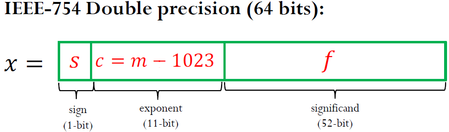
To achieve the range of values needed with the same number of bits, we use floating point numbers or float for short. Instead of utilizing each bit as the coefficient of a power of 2, floats allocate bits to three different parts: the sign indicator, \(s\), which says whether a number is positive or negative; characteristic or exponent, \(c\), which is the power of 2; and the fraction, \(f\), which is the coefficient of the exponent. Almost all platforms map Python floats to the IEEE754 double precision - 64 total bits. 1 bit is allocated to the sign indicator, 11 bits are allocated to the exponent, and 52 bits are allocated to the fraction. With 11 bits allocated to the exponent, this makes 2048 values that this number can take. Since we want to be able to make very precise numbers, we want some of these values to represent negative exponents (i.e., to allow numbers that are between 0 and 1 (base10)). To accomplish this, 1023 is subtracted from the exponent to normalize it. The value subtracted from the exponent is commonly referred to as the bias. The fraction is a number between 1 and 2. In binary, this means that the leading term will always be 1, and, therefore, it is a waste of bits to store it. To save space, the leading 1 is dropped.
Special values:
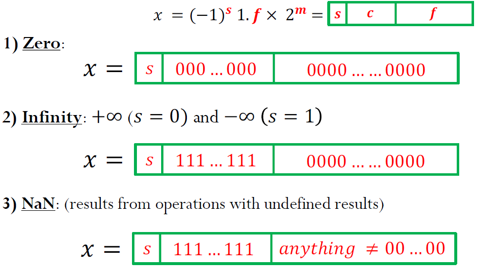
Note that the exponent \(c\) = 000…000 and \(c\) = 111…111 are reserved for these special cases, which limits the exponent range for the other numbers.
In Python, we could get the float information using the sys package as shown below:
import sys
sys.float_info
A float can then be represented as:
\(n = (-1)^s 2^{e-1023} (1+f).\) (for 64-bit)
Example: What is the number 1 10000000010 1000000000000000000000000000000000000000000000000000 (IEEE754) in base10?
The exponent in decimal is \(1 \cdot 2^{10} + 1 \cdot 2^{1} - 1023 = 3\). The fraction is \(1 \cdot \frac{1}{2^1} + 0 \cdot \frac{1}{2^2} + ... = 0.5\). Therefore \(n = (-1)^1 \cdot 2^{3} \cdot (1 + 0.5) = -12.0\) (base10).
Example: What is 15.0 (base10) in IEEE754? What is the largest number smaller than 15.0? What is the smallest number larger than 15.0?
Since the number is positive, \(s = 0\). The largest power of two that is smaller than 15.0 is 8,
so the exponent is 3, making the characteristic
\(3 + 1023 = 1026 (base10) = 10000000010(base2)\).
Then the fraction is
\(15/8-1=0.875(base10) = 1\cdot \frac{1}{2^1} + 1\cdot \frac{1}{2^2} + 1\cdot \frac{1}{2^3}\) = 1110000000000000000000000000000000000000000000000000 (base2).
When put together this produces the following conversion:
15 (base10) = 0 10000000010 1110000000000000000000000000000000000000000000000000 (IEEE754)
The next smallest number is 0 10000000010 1101111111111111111111111111111111111111111111111111 = 14.9999999999999982236431605997
The next largest number is 0 10000000010 1110000000000000000000000000000000000000000000000001 = 15.0000000000000017763568394003
Therefore, the IEEE754 number 0 10000000010 1110000000000000000000000000000000000000000000000000 not only represents the number 15.0, but also all the real numbers halfway between its immediate neighbors. So any computation that has a result within this interval will be assigned 15.0.
We call the distance from one number to the next the gap. Because the fraction is multiplied by \(2^{e-1023}\), the gap grows as the number represented grows. The gap at a given number can be computed using the function spacing in numpy.
import numpy as np
Example: Use the spacing function to determine the gap at 1e9. Verify that adding a number to 1e9 that is less than half the gap at 1e9 results in the same number.
np.spacing(1e9)
1e9 == (1e9 + np.spacing(1e9)/3)
There are special cases for the value of a floating point number when e = 0 (i.e., e = 00000000000 (base2)) and when e = 2047 (i.e., e = 11111111111 (base2)), which are reserved. When the exponent is 0, the leading 1 in the fraction takes the value 0 instead. The result is a subnormal number, which is computed by \(n=(-1)^s2^{-1022}(0+f)\) (note: it is -1022 instead of -1023). When the exponent is 2047 and f is nonzero, then the result is “Not a Number”, which means that the number is undefined. When the exponent is 2047, then f = 0 and s = 0, and the result is positive infinity. When the exponent is 2047, then f = 0, and s = 1, and the result is minus infinity.
Example: Compute the base10 value for 0 11111111110 1111111111111111111111111111111111111111111111111111 (IEEE754), the largest defined number for 64 bits, and for 0 00000000001 000000000000000000000000000000000000000000000000000 (IEEE754), the smallest. Note that the exponent is, respectively, e = 2046 and e = 1 to comply with the previously stated rules. Verify that Python agrees with these calculations using sys.float_info.max and sys.float_info.min.
largest = (2**(2046-1023))*((1 + sum(0.5**np.arange(1, 53))))
largest
sys.float_info.max
smallest = (2**(1-1023))*(1+0)
smallest
sys.float_info.min
Numbers that are larger than the largest representable floating point number result in overflow, and Python handles this case by assigning the result to inf. Numbers that are smaller than the smallest subnormal number result in underflow, and Python handles this case by assigning the result to 0.
Example: Show that adding the maximum 64 bits float number with 2 results in the same number. The Python float does not have sufficient precision to store the + 2 for sys.float_info.max, therefore, the operations is essentially equivalent to add zero. Also show that adding the maximum 64 bits float number with itself results in overflow and that Python assigns this overflow number to inf.
sys.float_info.max + 2 == sys.float_info.max
sys.float_info.max + sys.float_info.max
Example: The smallest subnormal number in 64-bit number has s = 0, e = 00000000000,
and
f = 0000000000000000000000000000000000000000000000000001. Using the special rules for subnormal numbers, this results in the
subnormal number \((-1)^02^{1-1023}2^{-52} = 2^{-1074}\). Show that
\(2^{-1075}\) underflows to 0.0 and that the result cannot be distinguished
from 0.0. Show that \(2^{-1074}\) does not.
2**(-1075)
2**(-1075) == 0
2**(-1074)
So, what have we gained by using IEEE754 versus binary? Using 64 bits binary gives us \(2^{64}\) numbers. Since the number of bits does not change between binary and IEEE754, IEEE754 must also give us \(2^{64}\) numbers. In binary, numbers have a constant spacing between them. As a result, you cannot have both range (i.e., large distance between minimum and maximum representable numbers) and precision (i.e., small spacing between numbers). Controlling these parameters would depend on where you put the decimal point in your number. IEEE754 overcomes this limitation by using very high precision at small numbers and very low precision at large numbers. This limitation is usually acceptable because the gap at large numbers is still small relative to the size of the number itself. Therefore, even if the gap is millions large, it is irrelevant to normal calculations if the number under consideration is in the trillions or higher.
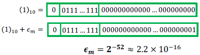
Machine epsilon \(\epsilon_{m}\)
Machine epsilon is defined as the distance (gap) between 1 and the next larger floating point number. In 64 bits
In Python one can get the machine epsilon with the following code:
def machineEpsilon():
    eps = 1.0
    while eps + 1.0 != 1.0:
        eps /= 2.0
    return eps
eps = machineEpsilon()
print("Machine epsilon: {}".format(eps))
Error in Numerical Methods
Every result we compute in Numerical Methods contain errors!. Our job is to reduce the impact of the errors. We model the error as:
Approximate result = True Value + Error
\(\hat{x} = x + \Delta x\)
Absolute error: \(E_{a} = \left |x - \hat{x} \right |\)
Relative error: \(E_{r} = \frac{\left |x - \hat{x} \right |}{x}\)
The relative error can also be multiplied by 100 percent to express it as the percent relative error: \[\varepsilon_{r} = \frac{\left |x - \hat{x} \right |}{x}*100 \%\]
The true value is rarely available in numerical methods. The true value will be known only when we deal with functions that can be solved analytically. In real-world applications, we will not know the true answer a priori. For these situations, an alternative is to normalize the error using the best available estimate of the true value (approximate error), that is, to the approximation itself, as in \[\varepsilon_{a} = \frac{approximate \hspace{1mm} error}{approximation}*100 \%\] where the subscript a signifies that the error is normalized to an approximate value.
One of the challenges of numerical methods is to determine error estimates
in the absence of knowledge regarding the true value. For example, certain numerical
methods use an iterative approach to compute answers. In such an approach, a present
approximation is made on the basis of a previous approximation. This process is performed
repeatedly, or iteratively, to successively compute better and better approximations.
For such cases, the error is often estimated as the difference between previous and
current approximations. Thus, percent relative error is determined according to
\[\varepsilon_{a} = \frac{current \hspace{1mm} approximation - previous \hspace{1mm} approximation}{current \hspace{1mm} approximation}*100 \%\]
when performing computations, we may not be concerned with the sign of the error, but we are interested
in whether the percent absolute value is lower than a prespecified percent tolerance \(\varepsilon_{s}\).
Therefore, it is often useful to employ the absolute value of \(\varepsilon_{a}\).
For such cases, the computation is repeated until
\(\left | \varepsilon_{a} \right | < \varepsilon_{s}\)
our result is assumed to be within the prespecified acceptable
level \(\varepsilon_{s}\).
It is also convenient to relate these errors to the number of significant figures in the
approximation. It can be shown (Scarborough, 1966) that if the following criterion is
met, we can be assured that the result is correct to at least n significant figures:
\( \varepsilon_{s} = (0.5 \times 10^{2 - n})\% \)
Significant digits
Significant figures of a number are digits that carry meaningful information. They are digits beginning to the leftmost nonzero digit and ending with the rightmost “correct” digit, including final zeros that are exact.
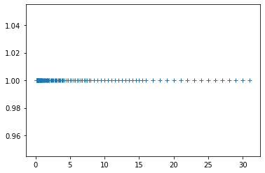
Example: Density of Floating Point Numbers
# # Density of Floating Point Numbers
# This example enumerates all possible floating point nubmers in a floating point system and shows them in a plot to illustrate their density.
import matplotlib.pyplot as pt
import numpy as np

significand_bits = 4
exponent_min = -3
exponent_max = 4

fp_numbers = []
for exp in range(exponent_min, exponent_max+1):
    for sbits in range(0, 2**significand_bits):
        significand = 1 + sbits/2**significand_bits
        fp_numbers.append(significand * 2**exp)

fp_numbers = np.array(fp_numbers)
print(fp_numbers)

pt.plot(fp_numbers, np.ones_like(fp_numbers), "+")
#pt.semilogx(fp_numbers, np.ones_like(fp_numbers), "+")
[ 0.125      0.1328125  0.140625   0.1484375  0.15625    0.1640625
  0.171875   0.1796875  0.1875     0.1953125  0.203125   0.2109375
  0.21875    0.2265625  0.234375   0.2421875  0.25       0.265625
  0.28125    0.296875   0.3125     0.328125   0.34375    0.359375
  0.375      0.390625   0.40625    0.421875   0.4375     0.453125
  0.46875    0.484375   0.5        0.53125    0.5625     0.59375
  0.625      0.65625    0.6875     0.71875    0.75       0.78125
  0.8125     0.84375    0.875      0.90625    0.9375     0.96875
  1.         1.0625     1.125      1.1875     1.25       1.3125
  1.375      1.4375     1.5        1.5625     1.625      1.6875
  1.75       1.8125     1.875      1.9375     2.         2.125
  2.25       2.375      2.5        2.625      2.75       2.875
  3.         3.125      3.25       3.375      3.5        3.625
  3.75       3.875      4.         4.25       4.5        4.75
  5.         5.25       5.5        5.75       6.         6.25
  6.5        6.75       7.         7.25       7.5        7.75
  8.         8.5        9.         9.5       10.        10.5
 11.        11.5       12.        12.5       13.        13.5
 14.        14.5       15.        15.5       16.        17.
 18.        19.        20.        21.        22.        23.
 24.        25.        26.        27.        28.        29.
 30.        31.       ]
Sources of Error
The Computational Error = \(\hat{f}(x) - f(x)\) = Truncation Error + Rounding Error
Main source of errors in numerical computation:
- Rounding error: occurs when digits in a decimal point (1/3 = 0.3333...) are lost (0.3333) due to a limit on the memory available for storing one numerical value. Rounding error is the error made due to inexact representation of quantities computed by the algorithm
- Truncation error: occurs when discrete values are used to approximate a mathematical expression (eg. the approximation sin 𝜃 ≈ 𝜃 for small angles 𝜃). Truncation error is the error made due to approximations made by the algorithm (simplified models used in our approximation), e.g. the representation of a function by a finite Taylor series \[f(x + h) \approx g(h) = \sum_{i=0}^{k}\frac{{f^{(i)}(x)}}{i!}h^{i} \] The absolute truncation error of this approximation is \[f(x + h) - g(h) = \sum_{i=k+1}^{\infty }\frac{{f^{(i)}(x)}}{i!}h^{i} = O(h^{k+1}) \hspace{1mm} as \hspace{1mm} h\rightarrow \infty \]
To study the propagation of roundooff error in arithmetic we can use the notion of conditioning. The condition number tells use the worst-case amplification of output error with respect to input error
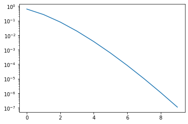
Example: Floating Point Arithmetic and the Series for the Exponential Function
What this example does is sum the series \[ \exp(x) \approx \sum_{i=0}^n \frac{x^i}{i!} \] for varying n , and varying x . It then prints the partial sum, the true value, and the final term of the series.
# # Floating Point Arithmetic and the Series for the Exponential Function
import numpy as np
import matplotlib.pyplot as pt

# What this example does is sum the series exp(x)
a = 0.0
x = 1e0 # flip sign
true_f = np.exp(x)
e = []

for i in range(0, 10): # crank up
    d = np.prod(
            np.arange(1, i+1).astype(np.float))
    # series for exp
    a += x**i / d
    print(a, np.exp(x), x**i / d)
    e.append(abs(true_f-a)/true_f)

pt.semilogy(e)
1.0 2.718281828459045 1.0
2.0 2.718281828459045 1.0
2.5 2.718281828459045 0.5
2.6666666666666665 2.718281828459045 0.16666666666666666
2.708333333333333 2.718281828459045 0.041666666666666664
2.7166666666666663 2.718281828459045 0.008333333333333333
2.7180555555555554 2.718281828459045 0.001388888888888889
2.7182539682539684 2.718281828459045 0.0001984126984126984
2.71827876984127 2.718281828459045 2.48015873015873e-05
2.7182815255731922 2.718281828459045 2.7557319223985893e-06
Example: Floating Point and the Harmonic Series
It is know from math that \[ \sum_{n=1}^\infty \frac 1n=\infty \] Let's see what we get using floating point:
# # Floating Point and the Harmonic Series
#
import numpy as np

n = int(0)
float_type = np.float32
my_sum = float_type(0)

while True:
    n += 1
    last_sum = my_sum
    my_sum += float_type(1 / n)

    if n % 200000 == 0:
        print("1/n = %g, sum0 = %g"%(1.0/n, my_sum))
Example: Picking apart a floating point number
# # Picking apart a floating point number
# Never mind the details of this function...

def pretty_print_fp(x):
    print("---------------------------------------------")
    print("Floating point structure for %r" % x)
    print("---------------------------------------------")
    import struct
    s = struct.pack("d", x)

    def get_bit(i):
        byte_nr, bit_nr = divmod(i, 8)
        return int(bool(
            s[byte_nr] & (1 << bit_nr)
            ))

    def get_bits(lsb, count):
        return sum(get_bit(i+lsb)*2**i for i in range(count))

    # https://en.wikipedia.org/wiki/Double_precision_floating-point_format

    print("Sign bit (1:negative):", get_bit(63))
    exponent = get_bits(52, 11)
    print("Stored exponent: %d" % exponent)
    print("Exponent (with offset): %d" % (exponent - 1023))
    fraction = get_bits(0, 52)
    if exponent != 0:
        significand = fraction + 2**52
    else:
        significand = fraction
    print("Significand (binary):", bin(significand)[2:])
    print("Shifted significand:", repr(significand / (2**52)))

pretty_print_fp(3)

# Things to try:
#
# * Twiddle the sign bit
# * 1,2,4,8
# * 0.5,0.25
# * $2^{\pm 1023}$, $2^{\pm 1024}$
# * `float("nan")`
Example: Floating Point Error in Horner's Rule Polynomial Evaluation
The following example is taken from Applied Numerical Linear Algebra by James Demmel, SIAM 1997.
Here are three methods for evaluating the function
\[f(x)=(x-2)^9 = -512 + 2304x -4608x^2 +5476x^3 -4032x^4 +2016x^5-672x^6+144x^7-18x^8+x^9 \]# ****Floating Point Error in Horner's Rule Polynomial Evaluation****
# The following example is taken from *Applied Numerical Linear Algebra* by James Demmel, SIAM 1997.
#
import numpy as np
#Evalue polynomial in factored form
def f(x):
return (x-2.)**9
#coefficients for expanded form
coeffs = np.asarray([-512., 2304., -4608., 5376., -4032., 2016., -672., 144., -18., 1.])
#Evaluate polynomial using coefficients
def p(x):
return np.inner(coeffs, np.asarray([x**i for i in range(10)]))
#Evaluate Horner's rule for polynomial
def h(x):
y = 0.
#[::-1] looks at all elements with stride -1, reversing the order
for c in coeffs[::-1]:
y = x*y+c
return y
#Define 8000 points between 1.92 and 2.08
xpts = 1.92+np.arange(8000.)/50000.
import matplotlib.pyplot as pt
#plot functions evaluated at each point using Horder's rule and using factored form
pt.plot(xpts,[h(x) for x in xpts],label='Evaluation by Horner\'s rule')
pt.plot(xpts,[f(x) for x in xpts],label='Evaluation in factored form')
pt.legend()
pt.show()
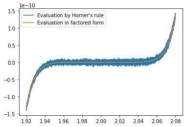
It seems Horner's rule is inaccurate when \(f(x)\approx 0\), lets try to understand why.
The first method uses \((x-2)^9\) directly, encurring a backward error of \(\epsilon\) (machine epsilon), since given \(z=\textit{fl}(x+2)\), we can obtain \(z^9\) to the same precision, therby solving the problem for \(\hat{x}=\textit{fl}(x+2)-2=x+ \Delta x\), \(|\Delta x|\leq \epsilon\).
The second uses the inner product formula \[f(x)=p(x)= \sum_{i=0}^9c_ix^i =\begin{bmatrix} -512 & 2304 & -4608 & 5476 & -4032 & 2016 & -672 & 144 & 18& 1 \end{bmatrix}\begin{bmatrix} 1\\ x \\ x^2 \\ x^3 \\ x^4 \\ x^5 \\ x^6 \\ x^7 \\ x^8 \\ x^9 \end{bmatrix}\]
The third uses Horner's rule, which requires fewer operations
\[f(x)=h(x) = c_0 + (c_1 + \ldots (c_8 + c_9x)x \ldots )x\]Each addition in the last two methods incurs a relative error of at most \(\epsilon\). An error in the innermost parenthesis, would correspond to evaluating the function at a slightly perturbed \(x\). However, the error in the summation done last, contributes directly to the result. When \(\left|f(x)\right|<|c_0|\epsilon\), the result will contain no accurate significant digits.
In terms of backward stability, extrapolating the above argument implies that the backward absolute error bound has the bound \[\textit{fl}(h(x))-f(x)=\Delta x \leq \epsilon \left(1+\left|\frac{df^{-1}}{dx}(x)\right|\right).\]
More generally, given their factorized form, we can evaluate any function with unconditional backward stability. But factorization is hard!
Example: Decimal module
The python decimal module provides support for decimal floating point arithmetic. By default it the module can already provide a 28 digits or more number and can interact with other python operations normally.
Simple example: 0.1 + 0.2 - 0.3
import decimal
a, b, c = 0.1, 0.2, 0.3

# ‘Decimal’ object instead of normal float type
dec_a = decimal.Decimal('0.1')
dec_b = decimal.Decimal('0.2')
dec_c = decimal.Decimal('0.3')
print('float a+b-c =',a+b-c)
print('decimal a+b-c =',dec_a+dec_b-dec_c)
Conditioning
Absolute Condition Number
The absolute condition number is a property of the problem, which measures its sensitivity to perturbations in input \[ \kappa_{abs}(f) = \lim_{size \hspace{1mm} of \hspace{1mm} input \hspace{1mm} perturbation\rightarrow 0}\hspace{2mm} \max_{inputs} \hspace{2mm} \max_{perturbations \hspace{1mm} in \hspace{1mm} inputs}\left | \frac{perturbation \hspace{1mm} in \hspace{1mm} output}{perturbation \hspace{1mm} in \hspace{1mm} input} \right | \] For problem f at input x it is simply the derivative of f at x, \[ \kappa_{abs}(f) = \lim_{\Delta x\rightarrow 0}\left | \frac{f(x+\Delta x)-f(x)}{\Delta x} \right | = \left | \frac{df}{dx} (x)\right | \] When considering a space of inputs \(\chi\) it is \[\kappa_{abs} = \textup{max}_{x\in \chi }\left | \frac{df}{dx} (x)\right | \]
(Relative) Condition Number
The relative condition number considers relative perturbations in input and output, so that \[ \kappa (f)=\kappa_{rel} (f) = \max_{x\in \chi }\lim_{\Delta x\rightarrow 0}\left | \frac{(f(x+\Delta x)-f(x))/f(x)}{\Delta x/x}\right |=\frac{\kappa_{abs} (f)\left | x \right |}{\left | f(x) \right |} \]
Posedness and Conditioning
What is the condition number of an ill-posed problem?
- If the condition number is bounded and the solution is unique, the problem is well-posed.
- An ill-posed problem \( f \) either has no unique solution or has a (relative) condition number of \( \kappa (f)= \infty \).
- This condition implies that the solutions to problem \( f \) are continuous and diferentiable in the given space of possible inputs to \( f \).
- Sometimes well-posedness is defined to only require continuity.
- Generally, \( \kappa (f)\) can be thought of as the reciprocal of the distance (in an appropriate geometric embedding of problem configurations) from \( f \) to the nearest ill-posed problem.
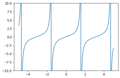
Example: Conditioning
# # Conditioning of evaluating tan()
import numpy as np
import matplotlib.pyplot as pt

# Let us estimate the sensitivity of evaluating the $\tan$ function:
x = np.linspace(-5, 5, 1000)
pt.ylim([-10, 10])
pt.plot(x, np.tan(x))

x = np.pi/2 - 0.0001
#x = 0.1
print(x)

print(np.tan(x))

dx = 0.00005
print(np.tan(x+dx))

# ## Condition number estimates
# ### From evaluation data
#
print(np.abs(np.tan(x+dx) - np.tan(x))/np.abs(np.tan(x)) / (np.abs(dx) / np.abs(x)))

# ### Using the derivative estimate

import sympy as sp

xsym = sp.Symbol("x")

f = sp.tan(xsym)
df = f.diff(xsym)
print(df)

# Evaluate the derivative estimate. Use `.subs(xsym, x)` to substitute in the value of `x`.

print((xsym*df/f).subs(xsym, x))
1.5706963267948966
9999.999966661644
19999.99998335545
31413.926693068603
tan(x)**2 + 1
15706.9633726542
Stability and Accuracy
Accuracy:
An algorithm is accurate if \( \hat{f}(x)=f(x) \) for all inputs \( x \) when \( \hat{f}(x) \) is computed in infinite precision
- In other words, the truncation error is zero (rounding error is ignored)
- More generally, an algorithm is accurate if its truncation error is negligible in the desired context
- Yet more generally, the accuracy of an algorithm is expressed in terms of bounds on the magnitude of its truncation error
Stability:
An algorithm is stable if its output in finite precision (floating point arithmetic) is always near its output in exact precision
- Stability measures the sensitivity of an algorithm to roundoff and truncation error
- In some cases, such as the approximation of a derivative using a finite difference formula, there is a trade-off between stability and accuracy
Rounding error in operations
Addition and Subtraction
- Subtraction is just negation of a sign bit followed by addition
- Catastrophic cancellation occurs when the magnitude of the result is much smaller than the magnitude of both operands
- Cancellation corresponds to losing significant digits
Multiplication and Division
- Multiplication is a lot safer than addition in floating point
- To analyze its error, we use a 2-term Taylor series approximation typical in relative error analysis
- Consequently, multiplication f(x, y) = xy is always well-conditioned, K(f)=3
- Division is multiplication by the reciprocal, and reciprocation is also well-conditioned
Example: Round-off error by floating-point arithmetic and Accumulation of round-off error
# Round-off error by floating-point arithmetic
print(4.9 - 4.845 == 0.055)

print(4.9 - 4.845)

print(4.8 - 4.845)

print(0.1 + 0.2 + 0.3 == 0.6)

# Accumulation of round-off error
# If we only do once
print(1 + 1/3 - 1/3)

def add_and_subtract(iterations):
    result = 1

    for i in range(iterations):
        result += 1/3

    for i in range(iterations):
        result -= 1/3
    return result

# If we do this 100 times
print(add_and_subtract(100))

# If we do this 1000 times
print(add_and_subtract(1000))

# If we do this 10000 times
print(add_and_subtract(10000))
Example: Catastrophic Cancellation
# # Catastrophic Cancellation
import numpy as np

# Let's make two numbers with very similar magnitude:
x = 1.48234
y = 1.48235

print(x-y)
# Now let's compute their difference in double precision:
x_dbl = np.float64(x)
y_dbl = np.float64(y)
diff_dbl = x_dbl-y_dbl

print(repr(diff_dbl))

# * What would the correct result be?
# -------------
# Can you predict what will happen in single precision?

x_sng = np.float32(x)
y_sng = np.float32(y)
diff_sng = x_sng-y_sng

print(diff_sng)
Example: Truncation Error vs Rounding Error
In this example, we'll investigate two common sources of error: Truncation error and rounding error.
# # Truncation Error vs Rounding Error
# In this example, we'll investigate two common sources of error: Truncation error and rounding error.
# **Task:** Approximate a function (here: a parabola, by a line)
import numpy as np
import matplotlib.pyplot as pt

center = -1
width = 6

def f(x):
    return - x**2 + 3*x

def df(x):
    return -2*x + 3

grid = np.linspace(center-width/2, center+width/2, 100)

fx = f(grid)
pt.plot(grid, fx)
pt.plot(grid, f(center) + df(center) * (grid-center))

pt.xlim([grid[0], grid[-1]])
pt.ylim([np.min(fx), np.max(fx)])
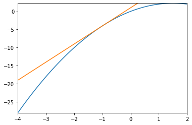
- What's the error we see?
- What if we make width smaller?
Example: Classical calculation of \(\pi\)
Approximating a circle by polygons (Liu Hui method)
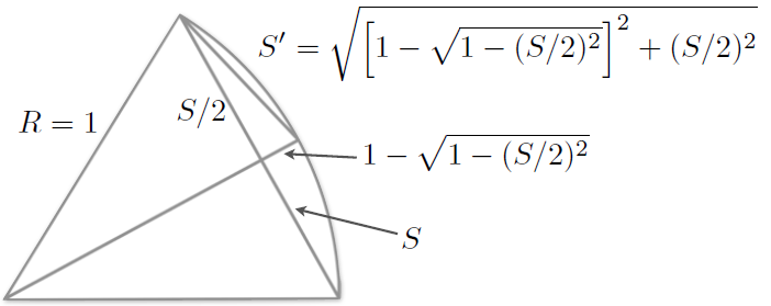
After many iterations: \[ \pi \approx \frac{S \times N_{sides}}{2}\]
import math
nsides = 6.
length = 1.
pi = length*nsides/2.
print('\t\t  sides',end='\t\t\t')
print('   S       ',end='\t\t\t')
print('pi(calc) ',end='\t\t')
print('diff pi(real-calc)')
print('%15.2f' %nsides,end='\t\t')
print('%.15f' % length,end='\t')
print('%.15f' % pi,end='\t')
print('%.15f' % abs(math.pi-pi))
for i in range(30):
    length = (2. - (4. - length**2)**0.5)**0.5
    nsides *= 2
    pi = length*nsides/2.
#    print('-'*30)
    print('%15.1f' %nsides,end='\t\t')
    print('%.15f' % length,end='\t')
    print('%.15f' % pi,end='\t')
    print('%.15f' % abs(math.pi-pi))
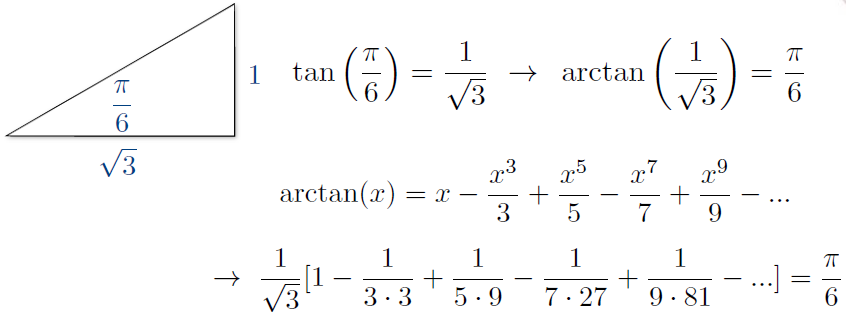
Example: Leibniz formula of \(\pi\)
Approximating trigonometric formula:
import math
print('step    \t pi(calc)    \t\t diff')
pi = 0.
numerator = 1./3.**0.5

for n in range(31):
    pi += numerator/(2.*n+1.)*6.
    numerator *= -1./3.
    print('%4d' % n,end='\t')
    print('%.15f' % pi,end='\t')
    print('%.15f' % abs(math.pi-pi))
Remark: How the errors behave
After N iterations of computing
- Approximation errors: In principle, the approximation (truncation) errors will be reduced if we go for more iterations (e.g. more terms in Taylor expansions).
- Roundoff errors: The roundoff error goes to the opposite direction, the more iterations, the error actually accumulates.


Limitation of the total error:
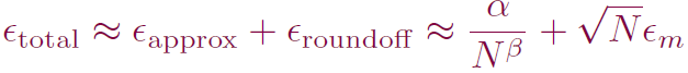
Example: \(\pi\) with Leibniz formula (ver. \(\pi\)/4): α ≈ 1, β ≈ 1 (since every 10x steps, we improve the calculation by 1 digit) If we do the calculation in double precision, when will we catch the smallest (critical) total error?
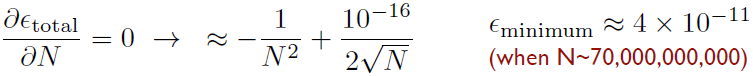
It's actually just a rough guesstimation, but it's always good to keep this idea in mind when you write your code!
The total numerical error is the summation of the truncation and round-off errors. In general, the only way to minimize round-off errors is to increase the number of significant figures of the computer. Further, the round-off error will increase due to subtractive cancellation or due to an increase in the number of computations in an analysis. In contrast, the truncation error can be reduced by decreasing the step size. Because a decrease in step size can lead to subtractive cancellation or to an increase in computations, the truncation errors are decreased as the round-off errors are increased. Therefore, we are faced by the following dilemma: The strategy for decreasing one component of the total error leads to an increase of the other component. In a computation, we could conceivably decrease the step size to minimize truncation errors only to discover that in doing so, the round-off error begins to dominate the solution and the total error grows! Thus, our remedy becomes our problem. One challenge that we face is to determine an appropriate step size for a particular computation. We would like to choose a large step size in order to decrease the amount of calculations and round-off errors without incurring the penalty of a large truncation error. If the total error is as shown in the following figure
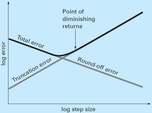
the challenge is to identify the point of diminishing returns where round-off error begins to negate the benefits of step-size reduction. In actual cases, however, such situations are relatively uncommon because most computers carry enough significant figures that round-off errors do not predominate. Nevertheless, they sometimes do occur and suggest a sort of "numerical uncertainty principle" that places an absolute limit on the accuracy that may be obtained using certain computerized numerical methods.
Example: Numerical derivatives
Suppose, you have a function f(x), and now you want to compute f’(x). By definition:
\[ f{}'(x)\approx \lim_{h\rightarrow 0}\frac{f(x + h) - f(x)}{h} \]In principle we could insert a small h, maybe as small as possible under the conversion of the numerical calculations. But this is not true for numerical derivatives.
Let's try such a simple function that we could actually do the exact calculations easily:
\[ f(x)=x^{2}+\exp (x)+\log (x) +\sin (x) \] \[\Rightarrow f{}'(x)=2x+\exp (x)+\frac{1}{x}+\cos (x)\]import math
def f(x):
return x**2+math.exp(x)+math.log(x)+math.sin(x)
def fp(x):
return 2.*x+math.exp(x)+1./x+math.cos(x)
# Starting from h = 1E-2
x, h = 0.5, 1E-2
fp_exact = fp(x)
print('Exact = %.16f\n' % fp_exact)
print ('\th \t\t Numerico \t\t diff')
while h>1E-15:
fp_numeric = (f(x+h) - f(x))/h
print('%.1e, ' % h, end=' ')
print('%.16f, ' % fp_numeric, end=' ')
print('%.16f' % abs(fp_numeric-fp_exact))
h /= 10. # retry with smaller h
import math

def f(x):
    return x**2+math.exp(x)+math.log(x)+math.sin(x)
def fp(x):
    return 2.*x+math.exp(x)+1./x+math.cos(x)

x, h = 0.5, 1E-2
fp_exact = fp(x)
print('Exact = %.16f\n' % fp_exact)
print ('  h \t    Numerico     \t       diff')
while h>1E-15:
    fp_numeric = (f(x+h/2.) - f(x-h/2.))/h
    print('%.0e, ' % h, end=' ')
    print('%.16f,' % fp_numeric, end=' ')
    print('%.16f' % abs(fp_numeric-fp_exact))
    h /= 10.
We can get a further improvement with the trick of “cancellation”:
\[ f{}'_{numerical}(x)\approx\frac{8f(x+\frac{h}{4}) -8f(x-\frac{h}{4}) - f(x+\frac{h}{2})+f(x-\frac{h}{2})}{3h} + \left [ O(h^{4})\cdots \right ]+O(\frac{\epsilon _{m}}{h}) \]
The total error \( \sim O(h^{4})+O(\frac{\epsilon _{m}}{h})\approx O(h^{4})+(\frac{10^{-16}}{h}) \)
The total error will saturation at: \( O(10^{-13})\) if \( h \approx O(\epsilon _{m}^{^{1/5}})\approx O(10^{-3}) \)
import math

def f(x):
    return x**2+math.exp(x)+math.log(x)+math.sin(x)
def fp(x):
    return 2.*x+math.exp(x)+1./x+math.cos(x)

x, h = 0.5, 1E-2
fp_exact = fp(x)
print('Exact = %.16f\n' % fp_exact)
print ('  h \t     Numerico    \t       diff')
while h>1E-15:
    fp_numeric = \
    (8.*f(x+h/4.)+f(x-h/2.)-8.*f(x-h/4.)-f(x+h/2.))/(h*3.)
    print('%.0e, ' % h, end=' ')
    print('%.16f,' % fp_numeric, end=' ')
    print('%.16f' % abs(fp_numeric-fp_exact))
    h /= 10.