## module linInterp
''' root = linInterp(f,x1,x2).
    Finds the zero of the linear function f(x) by straight
    line interpolation based on x = x1 and x2.
'''
def linInterp(f,x1,x2):
    f1 = f(x1)
    f2 = f(x2)
    return x2 - f2*(x2 - x1)/(f2 - f1)
## example8_1
# Solve the boundary value problem
# y'' + 3yy' = 0   y(0) = 0 y(2) = 1
import numpy as np
from run_kut4 import *
from ridder import *
from printSoln import *
def initCond(u): # Init. values of [y,y’]; use ’u’ if unknown
	return np.array([0.0, u])
def r(u): # Boundary condition residual--see Eq. (8.3)
	X,Y = integrate(F,xStart,initCond(u),xStop,h)
	y = Y[len(Y) - 1]
	r = y[0] - 1.0
	return r
def F(x,y): # First-order differential equations
	F = np.zeros(2)
	F[0] = y[1]
	F[1] = -3.0*y[0]*y[1]
	return F
xStart = 0.0 # Start of integration
xStop = 2.0 # End of integration
u1 = 1.0 # 1st trial value of unknown init. cond.
u2 = 2.0 # 2nd trial value of unknown init. cond.
h = 0.1 # Step size
freq = 2 # Printout frequency
u = ridder(r,u1,u2) # Compute the correct initial condition
X,Y = integrate(F,xStart,initCond(u),xStop,h)
printSoln(X,Y,freq)
input("\nPress return to exit")
## example8_3
# Solve the third-order boundary value problem
# y''' = 2y'' + 6xy    y(0) = 2 y(5) = y'(5) = 0
# and plot y and y' vs. x
import matplotlib.pyplot as plt
import numpy as np
from run_kut5 import *
from linInterp import *
def initCond(u): # Initial values of [y,y’,y"];
				# use ’u’ if unknown
	return np.array([0.0, 0.0, u])
def r(u): # Boundary condition residual--see Eq. (8.3)
	X,Y = integrate(F,xStart,initCond(u),xStop,h)
	y = Y[len(Y) - 1]
	r = y[0] - 2.0
	return r
def F(x,y): # First-order differential equations
	F = np.zeros(3)
	F[0] = y[1]
	F[1] = y[2]
	F[2] = 2.0*y[2] + 6.0*x*y[0]
	return F
xStart = 5.0 # Start of integration
xStop = 0.0 # End of integration
u1 = 1.0 # 1st trial value of unknown init. cond.
u2 = 2.0 # 2nd trial value of unknown init. cond.
h = -0.1 # initial step size
freq = 2 # printout frequency
u = linInterp(r,u1,u2)
X,Y = integrate(F,xStart,initCond(u),xStop,h)
plt.plot(X,Y[:,0],'o-',X,Y[:,1],'ˆ-')
plt.xlabel('x')
plt.legend(('y','dy/dx'),loc = 3)
plt.grid(True)
plt.show()
input("\nPress return to exit")
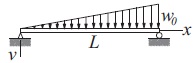
The displacement v of the simply supported beam can be obtained by solving the boundary value problem $$ \frac{d^{4}v}{dx^{4}}=\frac{w_{0}}{EI}\frac{x}{L} \;\;\;v=\frac{d^{2}v}{dx^{2}}=0 \;\; at \;\;x=0 \;\;and \;\;x=L $$ where E I is the bending rigidity. Determine by numerical integration the slopes at the two ends and the displacement at mid-span
## example8_4
# solving the boundary value problem
# d4v/dx4= w0 x/E IL   v = d2v/dx2= 0 at x = 0 and x = L
import numpy as np
from bulStoer import *
from newtonRaphson2 import *
from printSoln import *
def initCond(u): # Initial values of [y,y’,y",y"’];
				# use ’u’ if unknown
	return np.array([0.0, u[0], 0.0, u[1]])
def r(u): # Boundary condition residuals--see Eq. (8.7)
	r = np.zeros(len(u))
	X,Y = bulStoer(F,xStart,initCond(u),xStop,H)
	y = Y[len(Y) - 1]
	r[0] = y[0]
	r[1] = y[2]
	return r
def F(x,y): # First-order differential equations
	F = np.zeros(4)
	F[0] = y[1]
	F[1] = y[2]
	F[2] = y[3]
	F[3] = x
	return F
xStart = 0.0 # Start of integration
xStop = 1.0 # End of integration
u = np.array([0.0, 1.0]) # Initial guess for {u}
H = 0.5 # Printout increment
freq = 1 # Printout frequency
u = newtonRaphson2(r,u,1.0e-4)
X,Y = bulStoer(F,xStart,initCond(u),xStop,H)
printSoln(X,Y,freq)
input("\nPress return to exit")
Consider the differential equation $$ y^{(4)}+\frac{4}{x}y^{3}=0 $$ with the boundary conditions $$ y(0)={y}'(0)=0 \;\;\;\; {y}''(1)=0 \;\;\;\;{y}'''(1)=1 $$ Use numerical integration to determine y(1)
## example8_5
# Consider the differential equation
# y(4) + 4/x y3 = 0
# with the boundary conditions
# y(0) = y'(0) = 0 y''(1) = 0 y'''(1) = 1
# Use numerical integration to determine y(1).
import numpy as np
from run_kut5 import *
from newtonRaphson2 import *
from printSoln import *
def initCond(u): # Initial values of [y,y’,y",y"’];
	# use ’u’ if unknown
	return np.array([0.0, 0.0, u[0], u[1]])
def r(u): # Boundary condition residuals--see Eq. (8.7)
	r = np.zeros(len(u))
	X,Y = integrate(F,x,initCond(u),xStop,h)
	y = Y[len(Y) - 1]
	r[0] = y[2]
	r[1] = y[3] - 1.0
	return r
def F(x,y): # First-order differential equations
	F = np.zeros(4)
	F[0] = y[1]
	F[1] = y[2]
	F[2] = y[3]
	if x == 0.0: F[3] = -12.0*y[1]*y[0]**2
	else: F[3] = -4.0*(y[0]**3)/x
	return F
x = 0.0 # Start of integration
xStop = 1.0 # End of integration
u = np.array([-1.0, 1.0]) # Initial guess for u
h = 0.1 # Initial step size
freq = 0 # Printout frequency
u = newtonRaphson2(r,u,1.0e-5)
X,Y = integrate(F,x,initCond(u),xStop,h)
printSoln(X,Y,freq)
input("\nPress return to exit")
## example8_6
# Solve by finite difference method
# y'' = −4y + 4x    y(0) = 0    y'(π/2) = 0
import numpy as np
from LUdecomp3 import *
import math
def equations(x,h,m): # Set up finite difference eqs.
	h2 = h*h
	d = np.ones(m + 1)*(-2.0 + 4.0*h2)
	c = np.ones(m)
	e = np.ones(m)
	b = np.ones(m+1)*4.0*h2*x
	d[0] = 1.0
	e[0] = 0.0
	b[0] = 0.0
	c[m-1] = 2.0
	return c,d,e,b
xStart = 0.0 # x at left end
xStop = math.pi/2.0 # x at right end
m = 10 # Number of mesh spaces
h = (xStop - xStart)/m
x = np.arange(xStart,xStop + h,h)
c,d,e,b = equations(x,h,m)
c,d,e = LUdecomp3(c,d,e)
y = LUsolve3(c,d,e,b)
print("\n x \t y")
for i in range(m + 1):
	print('{:14.5e} {:14.5e}'.format(x[i],y[i]))
input("\nPress return to exit")
## example8_7
# Solve the boundary value problem
# y'' = −3yy'   y(0) = 0 y(2) = 1
# with the finite difference method. Use m = 10 and compare the output with the results
# of the shooting method in Example 8.1
import numpy as np
from newtonRaphson2 import *
def residual(y): # Residuals of finite diff. Eqs. (8.11)
	r = np.zeros(m + 1)
	r[0] = y[0]
	r[m] = y[m] - 1.0
	for i in range(1,m):
		r[i] = y[i-1] - 2.0*y[i] + y[i+1] \
		- h*h*F(x[i],y[i],(y[i+1] - y[i-1])/(2.0*h))
	return r
def F(x,y,yPrime): # Differential eqn. y" = F(x,y,y’)
	F = -3.0*y*yPrime
	return F
def startSoln(x): # Starting solution y(x)
	y = np.zeros(m + 1)
	for i in range(m + 1): y[i] = 0.5*x[i]
	return y
xStart = 0.0 # x at left end
xStop = 2.0 # x at right end
m = 10 # Number of mesh intervals
h = (xStop - xStart)/m
x = np.arange(xStart,xStop + h,h)
y = newtonRaphson2(residual,startSoln(x),1.0e-5)
print ("\n x \t \t y")
for i in range(m + 1):
	print ("%14.5e %14.5e" %(x[i],y[i]))
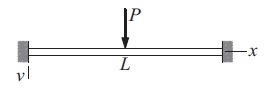
The uniform beam of length L and bending rigidity E I is attached to rigid supports at both ends. The beam carries a concentrated load P at its mid-span. If we utilize symmetry and model only the left half of the beam, the displacement v can be obtained by solving the boundary value problem $$ EI\frac{d^{4}v}{dx^{4}}=0 $$ $$ v|_{x=0}=0 \;\;\;\;\frac{dv}{dx}|_{x=0}=0 \;\;\;\;\frac{dv}{dx}|_{x=L/2}=0 \;\;\;\;EI\frac{d^{3}v}{dx^{3}}=-P/2 $$ Use the finite difference method to determine the displacement and the bending moment M = −E I d2v/dx2 at the mid-span
## example8_8
import numpy as np
from LUdecomp5 import *
def equations(x,h,m): # Set up finite difference eqs.
	h4 = h**4
	d = np.ones(m + 1)*6.0
	e = np.ones(m)*(-4.0)
	f = np.ones(m-1)
	b = np.zeros(m+1)
	d[0] = 1.0
	d[1] = 7.0
	e[0] = 0.0
	f[0] = 0.0
	d[m-1] = 7.0
	d[m] = 3.0
	b[m] = 0.5*h**3
	return d,e,f,b
xStart = 0.0 # x at left end
xStop = 0.5 # x at right end
m = 20 # Number of mesh spaces
h = (xStop - xStart)/m
x = np.arange(xStart,xStop + h,h)
d,e,f,b = equations(x,h,m)
d,e,f = LUdecomp5(d,e,f)
y = LUsolve5(d,e,f,b)
print('\n x y')
print('{:14.5e} {:14.5e}'.format(x[m-1],y[m-1]))
print('{:14.5e} {:14.5e}'.format(x[m],y[m]))
input("\nPress return to exit")