Chap7 Numerical methods Kiusalaas Python

## module euler
''' X,Y = integrate(F,x,y,xStop,h).
    Euler's method for solving the
    initial value problem {y}' = {F(x,{y})}, where
    {y} = {y[0],y[1],...y[n-1]}.
    x,y   = initial conditions
    xStop = terminal value of x
    h     = increment of x used in integration
    F     = user-supplied function that returns the
            array F(x,y) = {y'[0],y'[1],...,y'[n-1]}.
'''
import numpy as np
def integrate(F,x,y,xStop,h):    
    X = []
    Y = []
    X.append(x)
    Y.append(y)
    while x < xStop:
        h = min(h,xStop - x)
        y = y + h*F(x,y)
        x = x + h
        X.append(x)
        Y.append(y)
    return np.array(X),np.array(Y)

## module printSoln
''' printSoln(X,Y,freq).
    Prints X and Y returned from the differential
    equation solvers using printput frequency 'freq'.
        freq = n prints every nth step.
        freq = 0 prints initial and final values only.
'''
def printSoln(X,Y,freq):

    def printHead(n):
        print("\n        x  ",end=" ")
        for i in range (n):
            print("      y[",i,"] ",end=" ")
        print()

    def printLine(x,y,n):
        print("{:13.4e}".format(x),end=" ")
        for i in range (n):
            print("{:13.4e}".format(y[i]),end=" ")
        print()
    
    m = len(Y)
    try: n = len(Y[0])
    except TypeError: n = 1
    if freq == 0: freq = m
    printHead(n)
    for i in range(0,m,freq):
        printLine(X[i],Y[i],n)
    if i != m - 1: printLine(X[m - 1],Y[m - 1],n)

Integrate the initial value problem $$ {y}''=-0.1{y}'-x \:\:\:\:\:\:\: y(0)=0 \:\:\:\:\:\:\:{y}'(0)=1 $$ from x = 0 to 2 with Euler’s method using h = 0.05. Plot the computed y together with the analytical solution, $ y=100x-5x^{2}+990(e^{-0.1x}-1) $

import numpy as np
from euler import *
import matplotlib.pyplot as plt

def F(x,y):
	F = np.zeros(2)
	F[0] = y[1]
	F[1] = -0.1*y[1] - x
	return F
x = 0.0 # Start of integration
xStop = 2.0 # End of integration
y = np.array([0.0, 1.0]) # Initial values of {y}
h = 0.05 # Step size
X,Y = integrate(F,x,y,xStop,h)
yExact = 100.0*X - 5.0*X**2 + 990.0*(np.exp(-0.1*X) - 1.0)
plt.plot(X,Y[:,0],'o',X,yExact,'-')
plt.grid(True)
plt.xlabel('x'); plt.ylabel('y')
plt.legend(('Numerical','Exact'),loc=0)
plt.show()
input("Press return to exit")

## module run_kut4
''' X,Y = integrate(F,x,y,xStop,h).
    4th-order Runge-Kutta method for solving the
    initial value problem {y}' = {F(x,{y})}, where
    {y} = {y[0],y[1],...y[n-1]}.
    x,y   = initial conditions
    xStop = terminal value of x
    h     = increment of x used in integration
    F     = user-supplied function that returns the
            array F(x,y) = {y'[0],y'[1],...,y'[n-1]}.
'''
import numpy as np
def integrate(F,x,y,xStop,h):
    
    def run_kut4(F,x,y,h):
        K0 = h*F(x,y)
        K1 = h*F(x + h/2.0, y + K0/2.0)
        K2 = h*F(x + h/2.0, y + K1/2.0)
        K3 = h*F(x + h, y + K2)
        return (K0 + 2.0*K1 + 2.0*K2 + K3)/6.0    
    
    X = []
    Y = []
    X.append(x)
    Y.append(y)
    while x < xStop:
        h = min(h,xStop - x)
        y = y + run_kut4(F,x,y,h)
        x = x + h
        X.append(x)
        Y.append(y)
    return np.array(X),np.array(Y)

Integrate the initial value problem $$ {y}''=-0.1{y}'-x \:\:\:\:\:\:\: y(0)=0 \:\:\:\:\:\:\:{y}'(0)=1 $$ with the fourth-order Runge-Kutta method from x = 0 to 2 in increments of h = 0.2. Plot the computed y together with the analytical solution, $ y=100x-5x^{2}+990(e^{-0.1x}-1) $

Solution: Letting y₀ = y and y₁ = y', the equivalent first-order equations are $$F(x,y)=\begin{bmatrix} {y}_{0}'\\ {y}_{1}' \end{bmatrix} = \begin{bmatrix} y_{1}\\ -0.1y_{1}-x \end{bmatrix}$$

import numpy as np
from printSoln import *
from run_kut4 import *
import matplotlib.pyplot as plt

def F(x,y):
	F = np.zeros(2)
	F[0] = y[1]
	F[1] = -0.1*y[1] - x
	return F
x = 0.0 # Start of integration
xStop = 2.0 # End of integration
y = np.array([0.0, 1.0]) # Initial values of {y}
h = 0.2 # Step size
X,Y = integrate(F,x,y,xStop,h)
yExact = 100.0*X - 5.0*X**2 + 990.0*(np.exp(-0.1*X) - 1.0)
plt.plot(X,Y[:,0],'o',X,yExact,'-')
plt.grid(True)
plt.xlabel('x'); plt.ylabel('y')
plt.legend(('Numerical','Exact'),loc=0)
plt.show()
input("Press return to exit"))

Use the fourth-order Runge-Kutta method to integrate $$ {y}'=3y-4e^{-x} \;\;\;\;\; y(0)=1 $$ from x = 0 to 10 in steps of h = 0.1. Compare the result with the analytical solution $ y=e^{-x} $

## example7_5
import numpy as np
from run_kut4 import *
from printSoln import *
from math import exp
def F(x,y):
	F = np.zeros(1)
	F[0] = 3.0*y[0] - 4.0*exp(-x)
	return F
x = 0.0 # Start of integration
xStop = 10.0 # End of integration
y = np.array([1.0]) # Initial values of {y}
h = 0.1 # Step size
freq = 20 # Printout frequency
X,Y = integrate(F,x,y,xStop,h)
printSoln(X,Y,freq)
input("\nPress return to exit")

Example7_6: A spacecraft is launched at the altitude H = 772 km above sea level with the speed v₀ = 6700 m/s in the direction shown.

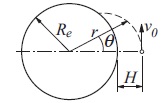
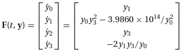
The differential equations describing the motion of the spacecraft are $$ \ddot{r}=r\dot{\theta }^{2}-\frac{GM_{e}}{r^{2}} \;\;\;\;\; \ddot{\theta }=-\frac{2\dot{r\dot{\theta }}}{r}$$ where r and θ are the polar coordinates of the spacecraft. The constants involved in the motion are
G = 6.672 × 10⁻¹¹ m³ kg⁻¹s⁻² = universal gravitational constant
M_e = 5.9742 × 1024 kg = mass of the earth
R_e = 6378.14 km = radius of the earth at sea level
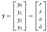
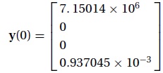
(1) Derive the first-order differential equations and the initial conditions of the form y' = F(t, y), y(0) = b.
(2) Use the fourth-order Runge-Kutta method to integrate the equations from the time of launch until the spacecraft hits the earth. Determine θ at the impact site

Solution:

## example7_6
import numpy as np
from run_kut4 import *
from printSoln import *
def F(x,y):
	F = np.zeros(4)
	F[0] = y[1]
	F[1] = y[0]*(y[3]**2) - 3.9860e14/(y[0]**2)
	F[2] = y[3]
	F[3] = -2.0*y[1]*y[3]/y[0]
	return F
x = 0.0
xStop = 1200.0
y = np.array([7.15014e6, 0.0, 0.0, 0.937045e-3])
h = 50.0
freq = 2
X,Y = integrate(F,x,y,xStop,h)
printSoln(X,Y,freq)
input("\nPress return to exit")

## module run_kut5
''' X,Y = integrate(F,x,y,xStop,h,tol=1.0e-6).
    Adaptive Runge-Kutta method with Dormand-Price
    coefficients for solving the
    initial value problem {y}' = {F(x,{y})}, where
    {y} = {y[0],y[1],...y[n-1]}.
    
    x,y   = initial conditions
    xStop = terminal value of x
    h     = initial increment of x used in integration
    tol   = per-step error tolerance
    F     = user-supplied function that returns the
            array F(x,y) = {y'[0],y'[1],...,y'[n-1]}.
'''
import math
import numpy as np

def integrate(F,x,y,xStop,h,tol=1.0e-6):
    
    a1 = 0.2; a2 = 0.3; a3 = 0.8; a4 = 8/9; a5 = 1.0
    a6 = 1.0
     
    c0 = 35/384; c2 = 500/1113; c3 = 125/192 
    c4 = -2187/6784; c5 = 11/84
         
    d0 = 5179/57600; d2 = 7571/16695; d3 = 393/640
    d4 = -92097/339200; d5 = 187/2100; d6 = 1/40
    
    b10 = 0.2
    b20 = 0.075; b21 = 0.225
    b30 = 44/45; b31 = -56/15; b32 = 32/9
    b40 = 19372/6561; b41 = -25360/2187; b42 = 64448/6561
    b43 = -212/729
    b50 = 9017/3168; b51 =-355/33; b52 = 46732/5247
    b53 = 49/176; b54 = -5103/18656
    b60 = 35/384; b62 = 500/1113; b63 = 125/192;
    b64 = -2187/6784; b65 = 11/84

    X = []
    Y = []
    X.append(x)
    Y.append(y)
    stopper = 0  # Integration stopper(0 = off, 1 = on)
    k0 = h*F(x,y)

    for i in range(10000):
        k1 = h*F(x + a1*h, y + b10*k0)
        k2 = h*F(x + a2*h, y + b20*k0 + b21*k1)
        k3 = h*F(x + a3*h, y + b30*k0 + b31*k1 + b32*k2)
        k4 = h*F(x + a4*h, y + b40*k0 + b41*k1 + b42*k2 + b43*k3)
        k5 = h*F(x + a5*h, y + b50*k0 + b51*k1 + b52*k2 + b53*k3 \
               + b54*k4)
        k6 = h*F(x + a6*h, y + b60*k0 + b62*k2 + b63*k3 + b64*k4 \
               + b65*k5)  
        
        dy = c0*k0 + c2*k2 + c3*k3 + c4*k4 + c5*k5
        E = (c0 - d0)*k0 + (c2 - d2)*k2 + (c3 - d3)*k3  \
               + (c4 - d4)*k4 + (c5 - d5)*k5 - d6*k6    
        e = math.sqrt(np.sum(E**2)/len(y))
        hNext = 0.9*h*(tol/e)**0.2
        
      # Accept integration step if error e is within tolerance
        if  e <= tol:
            y = y + dy
            x = x + h
            X.append(x)
            Y.append(y)  
            if stopper == 1: break  # Reached end of x-range
            if abs(hNext) > 10.0*abs(h): hNext = 10.0*h
            
          # Check if next step is the last one; if so, adjust h
            if (h > 0.0) == ((x + hNext) >= xStop):
                hNext = xStop - x
                stopper = 1
            k0 = k6*hNext/h
        else:
            if abs(hNext) < 0.1*abs(h): hNext = 0.1*h
            k0 = k0*hNext/h
        
        h = hNext
    return np.array(X),np.array(Y)

The aerodynamic drag force acting on a certain object in free fall can be approximated by $ F_{D}=av^{2}e^{-by} $ where
v = velocity of the object in m/s
y = elevation of the object in meters
a = 7.45 kg/m
b = 10.53 × 10⁻⁵ m⁻¹
The exponential term accounts for the change of air density with elevation. The differential equation describing the fall is where g = 9.806 65 m/s² and m = 114 kg is the mass of the object. If the object is released at an elevation of 9 km, determine its elevation and speed after a 10-s fall with the adaptive Runge-Kutta method.

Solution:

## example7_8
import numpy as np
import math
from run_kut5 import *
from printSoln import *
def F(x,y):
	F = np.zeros(2)
	F[0] = y[1]
	F[1] = -9.80665 + 65.351e-3 * y[1]**2 * math.exp(-10.53e-5*y[0])
	return F
x = 0.0
xStop = 10.0
y = np.array([9000, 0.0])
h = 0.5
freq = 1
X,Y = integrate(F,x,y,xStop,h,1.0e-2)
printSoln(X,Y,freq)
input("\nPress return to exit")

Integrate the moderately stiff problem
y'' = −19/4y − 10y' y(0) = −9 y'(0) = 0
from x = 0 to 10 with the adaptive Runge-Kutta method and plot the results

Solution:

## example7_9
import numpy as np
import matplotlib.pyplot as plt
from run_kut5 import *
from printSoln import *
def F(x,y):
	F = np.zeros(2)
	F[0] = y[1]
	F[1] = -4.75*y[0] - 10.0*y[1]
	return F
x = 0.0
xStop = 10.0
y = np.array([-9.0, 0.0])
h = 0.1
freq = 4
X,Y = integrate(F,x,y,xStop,h)
printSoln(X,Y,freq)
plt.plot(X,Y[:,0],'o-',X,Y[:,1],'ˆ-')
plt.xlabel('x')
plt.legend(('y','dy/dx'),loc=0)
plt.grid(True)
plt.show()
input("\nPress return to exit")

## module midpoint
''' yStop = integrate (F,x,y,xStop,tol=1.0e-6)
    Modified midpoint method for solving the
    initial value problem y' = F(x,y}.
    x,y   = initial conditions
    xStop = terminal value of x
    yStop = y(xStop)
    F     = user-supplied function that returns the
            array F(x,y) = {y'[0],y'[1],...,y'[n-1]}.
'''
import numpy as np
import math
def integrate(F,x,y,xStop,tol):

    def midpoint(F,x,y,xStop,nSteps):
        
  # Midpoint formulas
        h = (xStop - x)/nSteps
        y0 = y
        y1 = y0 + h*F(x,y0)
        for i in range(nSteps-1):
            x = x + h
            y2 = y0 + 2.0*h*F(x,y1)
            y0 = y1
            y1 = y2
        return 0.5*(y1 + y0 + h*F(x,y2))

    def richardson(r,k):
  # Richardson's extrapolation      
        for j in range(k-1,0,-1):
            const = (k/(k - 1.0))**(2.0*(k-j))
            r[j] = (const*r[j+1] - r[j])/(const - 1.0)
        return
    
    kMax = 51
    n = len(y)
    r = np.zeros((kMax,n))
  # Start with two integration steps
    nSteps = 2
    r[1] = midpoint(F,x,y,xStop,nSteps)
    r_old = r[1].copy()
  # Increase the number of integration points by 2
  # and refine result by Richardson extrapolation
    for k in range(2,kMax):
        nSteps = 2*k
        r[k] = midpoint(F,x,y,xStop,nSteps)
        richardson(r,k)
      # Compute RMS change in solution
        e = math.sqrt(np.sum((r[1] - r_old)**2)/n)
      # Check for convergence
        if e < tol: return r[1]
        r_old = r[1].copy()
    print("Midpoint method did not converge")

## module bulStoer
''' X,Y = bulStoer(F,x,y,xStop,H,tol=1.0e-6).
    Simplified Bulirsch-Stoer method for solving the
    initial value problem {y}' = {F(x,{y})}, where
    {y} = {y[0],y[1],...y[n-1]}.
    x,y   = initial conditions
    xStop = terminal value of x
    H     = increment of x at which results are stored
    F     = user-supplied function that returns the
            array F(x,y) = {y'[0],y'[1],...,y'[n-1]}.
'''
import numpy as np
from midpoint import *

def bulStoer(F,x,y,xStop,H,tol=1.0e-6):
    X = []
    Y = []
    X.append(x)
    Y.append(y)
    while x < xStop:
        H = min(H,xStop - x)
        y = integrate(F,x,y,x + H,tol) # Midpoint method
        x = x + H
        X.append(x)
        Y.append(y)
    return np.array(X),np.array(Y)

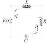
The differential equations governing the loop current i and the charge q on the capacitor of the electric circuit shown below are:
Ldi/dt+ Ri + q/C = E(t ) dq/dt= i
If the applied voltage E is suddenly increased from zero to 9 V, plot the resulting loop current during the first 10 s.
Use R = 1.0 Ω, L = 2 H, and C = 0.45 F. We solved the problem with the function bulStoer with the increment H = 0.25 s

Solution:

from bulStoer import *
import numpy as np
import matplotlib.pyplot as plt
def F(x,y):
F = np.zeros(2)
F[0] = y[1]
F[1] =(-y[1] - y[0]/0.45 + 9.0)/2.0
return F
H = 0.25
xStop = 10.0
x = 0.0
y = np.array([0.0, 0.0])
X,Y = bulStoer(F,x,y,xStop,H)
plt.plot(X,Y[:,1],'o-')
plt.xlabel('Time (s)')
plt.ylabel('Current (A)')
plt.grid(True)
plt.show()
input("\nPress return to exit")