## module trapezoid
''' Inew = trapezoid(f,a,b,Iold,k).
    Recursive trapezoidal rule:
    Iold = Integral of f(x) from x = a to b computed by
    trapezoidal rule with 2^(k-1) panels.
    Inew = Same integral computed with 2^k panels.
'''
def trapezoid(f,a,b,Iold,k):
    if k == 1:Inew = (f(a) + f(b))*(b - a)/2.0
    else:
        n = 2**(k -2 )      # Number of new points
        h = (b - a)/n       # Spacing of new points
        x = a + h/2.0       # Coord. of 1st new point
        sum = 0.0
        for i in range(n):
            sum = sum + f(x)
            x = x + h
        Inew = (Iold + h*sum)/2.0
    return Inew
## example6_4
# Use the recursive trapezoidal rule to evaluate
# int_0_π
# sqrt(x) cosx dx to six decimal places and determine
# how many panels are needed to achieve this result
import math
from trapezoid import *
def f(x): return math.sqrt(x)*math.cos(x)
Iold = 0.0
for k in range(1,21):
	Inew = trapezoid(f,0.0,math.pi,Iold,k)
	if (k > 1) and (abs(Inew - Iold)) < 1.0e-6: break
	Iold = Inew
print("Integral =",Inew)
print("nPanels =",2**(k-1))
input("\nPress return to exit")
## module romberg
''' I,nPanels = romberg(f,a,b,tol=1.0e-6).
    Romberg intergration of f(x) from x = a to b.
    Returns the integral and the number of panels used.
'''
import numpy as np
from trapezoid import *

def romberg(f,a,b,tol=1.0e-6):

    def richardson(r,k):
        for j in range(k-1,0,-1):
            const = 4.0**(k-j)
            r[j] = (const*r[j+1] - r[j])/(const - 1.0)
        return r

    r = np.zeros(21)
    r[1] = trapezoid(f,a,b,0.0,1)
    r_old = r[1]
    for k in range(2,21):
        r[k] = trapezoid(f,a,b,r[k-1],k)
        r = richardson(r,k)
        if abs(r[1]-r_old) < tol*max(abs(r[1]),1.0):
            return r[1],2**(k-1)
        r_old = r[1]
    print("Romberg quadrature did not converge")
Use Romberg integration to evaluate \(\int_{0}^{\sqrt{\pi }}2x^{2}\,\textup{cos}\,x^{2}\:dx \)
## example6_7
# Use Romberg integration to evaluate integ_0_√π  2x^2 cos x^2 dx
import math
from romberg import *
def f(x): return 2.0*(x**2)*math.cos(x**2)
I,n = romberg(f,0,math.sqrt(math.pi))
print("Integral =",I)
print("numEvals =",n)
input("\nPress return to exit")
## module gaussNodes
''' x,A = gaussNodes(m,tol=10e-9)
    Returns nodal abscissas {x} and weights {A} of
    Gauss-Legendre m-point quadrature.
'''
import math
import numpy as np

def gaussNodes(m,tol=10e-9):

    def legendre(t,m):
        p0 = 1.0; p1 = t
        for k in range(1,m):
            p = ((2.0*k + 1.0)*t*p1 - k*p0)/(1.0 + k )
            p0 = p1; p1 = p
        dp = m*(p0 - t*p1)/(1.0 - t**2)
        return p,dp

    A = np.zeros(m)
    x = np.zeros(m)
    nRoots = int((m + 1)/2)         # Number of non-neg. roots
    for i in range(nRoots):
        t = math.cos(math.pi*(i + 0.75)/(m + 0.5))# Approx. root
        for j in range(30):
            p,dp = legendre(t,m)    # Newton-Raphson
            dt = -p/dp; t = t + dt  # method
            if abs(dt) < tol:
                x[i] = t; x[m-i-1] = -t
                A[i] = 2.0/(1.0 - t**2)/(dp**2) # Eq.(6.25)
                A[m-i-1] = A[i]
                break
    return x,A
## module gaussQuad
''' I = gaussQuad(f,a,b,m).
    Computes the integral of f(x) from x = a to b
    with Gauss-Legendre quadrature using m nodes.
'''
from gaussNodes import *

def gaussQuad(f,a,b,m):
    c1 = (b + a)/2.0
    c2 = (b - a)/2.0
    x,A = gaussNodes(m)
    sum = 0.0
    for i in range(len(x)):
        sum = sum + A[i]*f(c1 + c2*x[i])
    return c2*sum
Determine how many nodes are required to evaluate \(\int_{a}^{\pi }\left ( \frac{\textup{sin}\,x}{x} \right )^{2}\:dx\) with Gauss-Legendre quadrature to six decimal places. The exact integral, rounded to six places, is 1.41815
import math
from gaussQuad import *
def f(x): return (math.sin(x)/x)**2
a = 0.0; b = math.pi;
Iexact = 1.41815
for m in range(2,12):
	I = gaussQuad(f,a,b,m)
	if abs(I - Iexact) < 0.00001:
		print("Number of nodes =",m)
		print("Integral =", gaussQuad(f,a,b,m))
		break
input("\nPress return to exit")
## module gaussQuad2
''' I = gaussQuad2(f,xc,yc,m).
    Gauss-Legendre integration of f(x,y) over a
    quadrilateral using integration order m.
    {xc},{yc} are the corner coordinates of the quadrilateral.
'''
from gaussNodes import *
import numpy as np
def gaussQuad2(f,x,y,m):

    def jac(x,y,s,t):
        J = np.zeros((2,2))
        J[0,0] = -(1.0 - t)*x[0] + (1.0 - t)*x[1]  \
                + (1.0 + t)*x[2] - (1.0 + t)*x[3]
        J[0,1] = -(1.0 - t)*y[0] + (1.0 - t)*y[1]  \
                + (1.0 + t)*y[2] - (1.0 + t)*y[3]
        J[1,0] = -(1.0 - s)*x[0] - (1.0 + s)*x[1]  \
                + (1.0 + s)*x[2] + (1.0 - s)*x[3]
        J[1,1] = -(1.0 - s)*y[0] - (1.0 + s)*y[1]  \
                + (1.0 + s)*y[2] + (1.0 - s)*y[3]
        return (J[0,0]*J[1,1] - J[0,1]*J[1,0])/16.0

    def map(x,y,s,t):
        N = np.zeros(4)
        N[0] = (1.0 - s)*(1.0 - t)/4.0
        N[1] = (1.0 + s)*(1.0 - t)/4.0
        N[2] = (1.0 + s)*(1.0 + t)/4.0
        N[3] = (1.0 - s)*(1.0 + t)/4.0
        xCoord = np.dot(N,x)
        yCoord = np.dot(N,y)
        return xCoord,yCoord

    s,A = gaussNodes(m)
    sum = 0.0
    for i in range(m):
        for j in range(m):
            xCoord,yCoord = map(x,y,s[i],s[j])
            sum = sum + A[i]*A[j]*jac(x,y,s[i],s[j])  \
                       *f(xCoord,yCoord)
    return sum
Use gaussQuad2 to evaluate \(\iint_{A}^{}f(x,y)\,dx\, dy \) over the quadrilateral shown below where \(f(x)= (x-2)^{2}(y-2)^{2} \). Use enough integration points for an "exact" answer
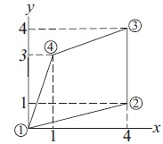
from gaussQuad2 import *
import numpy as np
def f(x,y): return ((x - 2.0)**2)*((y - 2.0)**2)
x = np.array([0.0, 4.0, 4.0, 1.0])
y = np.array([0.0, 1.0, 4.0, 3.0])
m = eval(input("Integration order ==> "))
print("Integral =", gaussQuad2(f,x,y,m))
input("\nPress return to exit")
## module triangleQuad
''' integral = triangleQuad(f,xc,yc).
    Integration of f(x,y) over a triangle using
    the cubic formula.
    {xc},{yc} are the corner coordinates of the triangle.
'''
import numpy as np

def triangleQuad(f,xc,yc):
    alpha = np.array([[1.0/3, 1.0/3.0, 1.0/3.0],  \
                      [0.2, 0.2, 0.6],            \
                      [0.6, 0.2, 0.2],            \
                      [0.2, 0.6, 0.2]])
    W = np.array([-27.0/48.0,25.0/48.0,25.0/48.0,25.0/48.0])
    x = np.dot(alpha,xc)
    y = np.dot(alpha,yc)
    A = (xc[1]*yc[2] - xc[2]*yc[1]      \
       - xc[0]*yc[2] + xc[2]*yc[0]      \
       + xc[0]*yc[1] - xc[1]*yc[0])/2.0
    sum = 0.0
    for i in range(4):
        sum = sum + W[i] * f(x[i],y[i])
    return A*sum
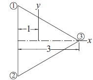
Evaluate \(\iint_{A}^{}f(x,y)\,dx\, dy \) over the equilateral triangle shown below where \(f(x)= \frac{1}{2}(x^{2}+y^{2})-\frac{1}{6}(x^{3}-3xy^{2})-\frac{2}{3} \). Use the quadrature formulas for (1) a quadrilateral and (2) a triangle
## example6_16a
from gaussQuad2 import *
import numpy as np
import math
def f(x,y):
	return (x**2 + y**2)/2.0 \
		- (x**3 - 3.0*x*y**2)/6.0 \
		- 2.0/3.0
x = np.array([-1.0,-1.0,2.0,2.0])
y = np.array([math.sqrt(3.0),-math.sqrt(3.0),0.0,0.0])
m = eval(input("Integration order ==> "))
print("Integral =", gaussQuad2(f,x,y,m))
input("\nPress return to exit")


## example6_16b
import numpy as np
import math
from triangleQuad import *
def f(x,y):
	return (x**2 + y**2)/2.0 \
		-(x**3 - 3.0*x*y**2)/6.0 \
		-2.0/3.0
xCorner = np.array([-1.0, -1.0, 2.0])
yCorner = np.array([math.sqrt(3.0), -math.sqrt(3.0), 0.0])
print("Integral =",triangleQuad(f,xCorner,yCorner))
input("Press return to exit")
<